
Ok, this doesn’t happen every day, but when it does…
By colin on Thursday, October 3rd, 2024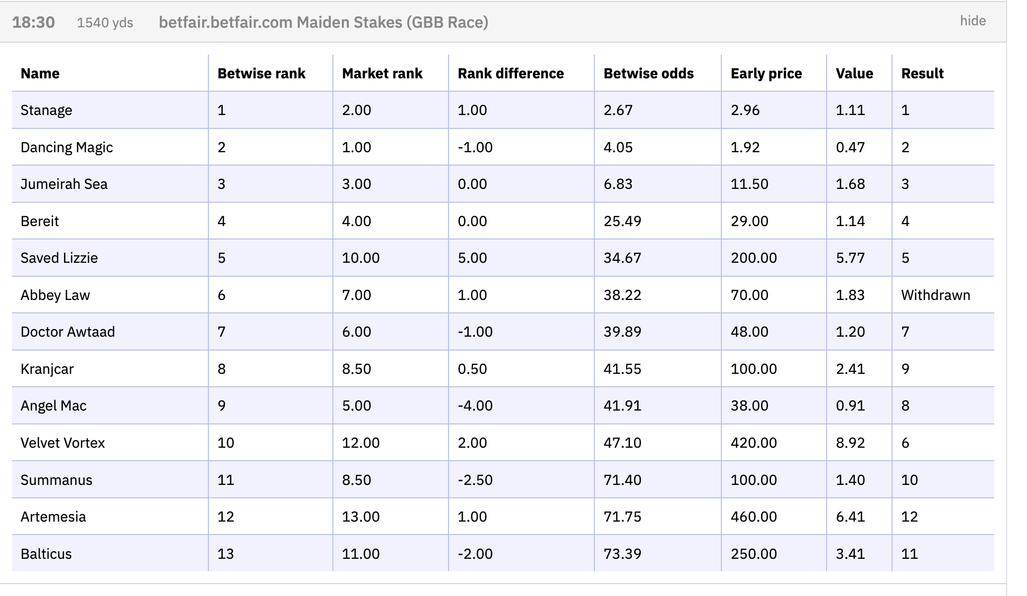
In the screenshot bove, we see key metrics from the Betwise Daily Oddsline service. Here’s a quick breakdown of what each represents:
- Name: The horse’s name.
- Betwise rank: A ranking assigned by the Betwise algorithm based on the horse’s predicted chances of winning.
- Market rank: The ranking according to the betting market’s early prices.
- Rank difference: The difference between Betwise rank and market rank, highlighting where Betwise disagrees with the market.
- Betwise odds: The odds predicted by the Betwise model, reflecting its calculation of each horse’s winning probability.
- Early price: The early market odds available on Betfair.
- Value: The ratio of early price to Betwise odds, showing potential value for bettors.
- Result: The horse’s actual finishing position. (Of course, when odds are posted before the race, this column is empty! But after the result is updated, nothing changes.)
This race was run just a few hours ago, and while we don’t see outcomes this perfect every time, the Betwise rankings aligned almost perfectly with the race result, right to the smallest places. You’d not have made much money with this prediction, but it’s notable that Saved Lizzie, ranked 5th by the oddsline, was only ranked 10th by the market, hence a big price discrepancy, almost 6 times the Betwise price, despite finishing exactly where predicted, in 5th place.
The strong correlation between the Betwise rank and actual race outcomes highlights the power of the Oddsline’s approach. By leveraging statistical models and machine learning, it captures the critical factors needed to provide value without relying on the market. As we discussed in this week’s earlier blog post, this data-driven method offers insights you won’t find elsewhere.
If you’re looking to sharpen your betting strategy with a data-driven perspective, you can sign up for the Betwise Oddsline here.
Harnessing Machine Learning for Smarter Market Insights with the Betwise Odds Line
By colin on Wednesday, October 2nd, 2024The modern horse racing landscape has evolved significantly with the introduction of technology-driven tools that enable bettors and analysts to make more informed decisions. 15 years ago we wrote about how to harness the value of a machine learning driven oddsline in the book Automatic Exchange Betting. For over four years, we offered a free daily oddsline for all types of thoroughbred horse racing in the UK and Ireland. We’ve been continually improving the Betwise Odds Line, and with the latest version—now available as a low-cost subscription service—we have developed an advanced, machine learning-driven tool that not only offers a solid foundation for race analysis but also offers a form driven perspective on the marke. As we continue to refine and enhance this tool, our mission with the oddsline is to help subscribers identify opportunities and navigate the more uncertain areas of the betting landscape.
The Betwise Odds Line is powered by the SmartForm database. The database itself provides all the raw data needed to build your own models, and we use it ourselves for the oddsline process. That process begins with feature engineering, and we have now created and tested a feature universe of over 700 derived variables for this purpose. These variables cover every conceivable angle, from a horse’s past performance to trainer, jockey and sire statistics as well as our own proprietary speed ratings, creating a rich dataset that drives our machine learning algorithms. Users of the Smartform database are able to do this for themseleves and in many cases build their own models. In our case, this comprehensive data set goes into models aimed at predicting the probability of a horse winning a race. The objective is to enable the Betwise Odds Line to offer a consistent, objective, and powerful approach to understanding race probabilities. By training on this vast amount of information, our model can rank horses in terms of probability of winning, with forecast probabilities or odds for each contender. This data – the oddsline – can then be used to identify where the market might be overestimating or underestimating a contender’s chances, or indeed where the market clearly diverges with the oddsline, and may “know” something pure form cannot reveal. This makes the odds line not just a foundation, but a strategic tool that can reveal genuine opportunities and those horses with the strongest probabilities of winning any given race. Beyond that, since this is not a “tipster” service, we can look at the structure of any given market versus the oddsline, and consider how the ranking order produced by the oddsline can be used to identify value in place bets, forecasts, tricasts and multiples – or pool bets, such as the placepot.
While the Betwise Odds Line excels in providing a robust data-driven foundation, we are completely aware of the inherent uncertainties in predicting outcomes. There are always factors that form data cannot fully capture — the form database has no knowledge of home gallops, horse improvement or deterioration off the track, trainers and owners “plots”, horses acting up on the way to the post, the unpredictable nature of the race itself and so on – all of which will alter the dynamics of the race and the probability that any horse has of winning. These are the nuances that make betting both challenging and intriguing, and this uncertainty will often be mirrored in fluctuating market odds and rankings. Our ongoing development efforts focus on highlighting where the odds line’s predictions might be more or less confident, and it’s important to note that the oddsline does not use any market information. This opens up new avenues for understanding how market pricing compares to raw race probabilities. In fact, both the more confident predictions and the fuzzier areas can present opportunities. By understanding where the odds line is most accurate and where it’s more uncertain, as well as where the market may be more influential, bettors can tailor their strategies accordingly, exploring these subtleties to find value that others might miss.
Since launching the Betwise Odds Line, we’ve now added live results, allowing you to track performance in real time. We will soon be adding tote returns and live pools, enhancing the ability to use the oddsline for deeper race analysis, particularly where ranking order within the race is paramount for exotic bet strategies. Not to mention providing rankings to help navigate a whole meeting.
As we continue to refine the service, our goal is to make it an indispensable tool for bettors. By subscribing, you’re not just gaining access to a an oddsline—you’re joining a service dedicated to exploring the complexities of horse racing and probability. Our journey is about more than just offering probabilities; it’s about understanding the dynamics of horse racing markets and providing you with the insights to make smarter, more informed decisions. Whether you’re seeking clear-cut value or eager to explore the sport’s fascinating uncertainties, join us as we push the boundaries of data-driven insights for smarter market strategies.
You can find out more here and sign up at: Betwise Odds Line.
Introducing GitHub
By Henry Young on Tuesday, May 14th, 2024Betwise has created an area on GitHub for Smartform community members to share their ideas, code, etc:
https://github.com/Betwise-Smartform
GitHub is one the most popular sites for hosting open source software and other types of shared information. I have kicked things off by uploading a simplified version of a race card tool I built using Excel/VBA:
https://github.com/Betwise-Smartform/ExcelCard
In my next blog post I’ll outline some of the techniques used to get data from Smartform into Excel using VBA (Visual Basic for Applications) to query the database. Then in subsequent blog posts I’ll add a variety of interesting predictive statistics columns that will turn the race card into a handy tool for analyzing races.
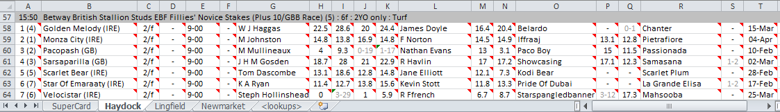
Eventually we’ll end up with the race card that I use daily to inform my own betting selections. Here’s an example of the 15:50 at Haydock on 7 June 2020, won by Golden Melody with Velocistar coming in last. My selection was to lay Velocistar. I won’t go into the details of what these columns are just yet, but a quick eyeball of the various numbers (mostly % strike rates aggregated in various ways) shows big numbers for Golden Melody and small numbers for Velocistar, suggesting back and lay opportunities respectively. Click on the image to blow it up.
As we progress through the series, I hope this will inspire you to try out some of the ideas, contribute back your own improvements and even create new GitHub repositories yourself to share your own work with the Smartform community.
Pat Cosgrave’s 28 Day Ban
By Henry Young on Saturday, April 22nd, 2023You may have seen that Pat Cosgrave received a 28 day ban for easing what should have been an easy winner on Concord in the Chelmsford 8pm on 20th April 2023. You can read the Racing Post report here:
Of immediate interest to me is why did he do this? While some may suggest dubious intent, my first thought was that as a seasoned jockey, and given the insights into jockey changing room culture that leak out from time to time, perhaps he simply enjoys underlining his seniority there with over the shoulder glances and a “look at me winning with no hands” attitude which he simply misjudged on this occasion. So I wanted to re-watch some of his other big distance wins to assess his riding manner in similar situations.
But how to find these easy win races ?
Smartform to the rescue with a simple SQL query:
mysql> select scheduled_time, name, course, finish_position as position, distance_won as distance from historic_runners_beta join historic_races_beta using (race_id) where jockey_name = "P Cosgrave" and finish_position = 1 order by distance_won desc limit 20;
+---------------------+--------------------+---------------+----------+----------+
| scheduled_time      | name               | course        | position | distance |
+---------------------+--------------------+---------------+----------+----------+
| 2022-07-07 17:53:00 | Caius Chorister    | Epsom_Downs   |        1 |    19.00 |
| 2006-07-18 19:10:00 | Holdin Foldin      | Newcastle     |        1 |    17.00 |
| 2003-10-25 17:00:00 | Excalibur          | Curragh       |        1 |    15.00 |
| 2015-05-20 14:30:00 | Wonder Laish       | Lingfield     |        1 |    15.00 |
| 2015-10-06 14:10:00 | Light Music        | Leicester     |        1 |    14.00 |
| 2009-01-29 14:20:00 | More Time Tim      | Southwell     |        1 |    13.00 |
| 2018-07-19 14:20:00 | Desert Fire        | Leicester     |        1 |    12.00 |
| 2008-12-12 12:55:00 | Confucius Captain  | Southwell     |        1 |    10.00 |
| 2010-04-27 16:10:00 | On Her Way         | Yarmouth      |        1 |    10.00 |
| 2018-09-22 15:55:00 | Stars Over The Sea | Newmarket     |        1 |    10.00 |
| 2012-10-25 16:40:00 | Saaboog            | Southwell     |        1 |     9.00 |
| 2006-03-31 15:40:00 | John Forbes        | Musselburgh   |        1 |     8.00 |
| 2015-05-20 15:00:00 | I'm Harry          | Lingfield     |        1 |     8.00 |
| 2018-06-17 15:10:00 | Pirate King        | Doncaster     |        1 |     8.00 |
| 2019-05-19 17:30:00 | Great Example      | Ripon         |        1 |     8.00 |
| 2004-07-19 18:30:00 | Orpailleur         | Ballinrobe    |        1 |     7.00 |
| 2007-07-04 17:35:00 | Serena's Storm     | Catterick     |        1 |     7.00 |
| 2008-01-07 13:50:00 | Home               | Southwell     |        1 |     7.00 |
| 2014-09-06 20:50:00 | Fiftyshadesfreed   | Wolverhampton |        1 |     7.00 |
| 2015-05-16 13:45:00 | Firmdecisions      | Newmarket     |        1 |     7.00 |
+---------------------+--------------------+---------------+----------+----------+
20 rows in set (5.55 sec)
You can watch the top race here, with no apparent easing but plenty of glances behind:
The point of this article is really to emphasize that with Smartform and a modicum of SQL knowledge, you can easily answer those oddball questions that come up from time to time, that no existing software solution or website will answer as easily.
Improvements to advance racecards in Smartform
By colin on Sunday, March 12th, 2023The daily_racecards and daily_runners tables have always provided racecards as early as they were available (usually two days ahead of the meetings, but for big races sometimes as many as five days ahead).
This provides benefits for users doing advance race analysis but presents some issues in ensuring that the most up-to-date cards are available – for example, reflecting latest non-runners, jockey changes, or race time changes – in daily cards
Improvements
To improve both use cases from now on, the daily_racecards and daily_runners tables (and their equivalent in the beta database) will provide new racecards only on the evening before the meetings, so they will always carry the final declarations.
To complement this and enable analysis more than 24 hours before racing, we have added new database feeds with equivalent tables to daily* for advance racecards for both the original and beta database products. These two feeds will provide the card on the first available day it is available to us, usually up to two days in advance, or more for big race meetings.
Making it all work for your subscription
daily* tables
There is nothing that you need to do in order to keep receiving daily updates, and in fact your database will now receive more up to date information (reflecting the final declarations) for the next day. However, these tables will no longer contain any data more than one day in advance of the race. If you want tomorrow’s cards earlier than 7.30 pm the day before the race, or the cards for racing the day after tomorrow, look to advance race cards, as below…
advance* tables
To receive the advance* data, you can jump straight to download details for the individual products at the following links:
Original database: https://www.betwise.co.uk/smartform/advance_racecards
Beta database: https://www.betwise.co.uk/smartform/advance_racecards_beta
So for the upcoming Cheltenham meeting, for example, you will soon see the earliest cards for advance analysis in the advance* tables, and the most up to date cards in the daily* tables the evening before racing.
The Johnstons : Mark > Mark & Charlie > Charlie
By Henry Young on Friday, February 10th, 2023The Johnstons have become a racing dynasty. Mark Johnston first registered his trainer’s license in 1987. In 2009 he became the first flat trainer to send out more than 200 winners in a single season (2009). He went on to repeat that feat in 2010, 2012, 2013, 2014, 2015, 2017, 2018, 2019 and 2021. His son Charlie was brought up to follow in his father’s footsteps and take over the family business. He started working full time for Mark in 2016, and joined his father on their joint trainers license in late January 2022, with Mark leaving the license from January 2023.
The key question for us is what implication does this have for the data in the Smartform database. Let’s take a look at the trainer_id values:
select distinct trainer_name, trainer_id from historic_runners_beta where trainer_name like "%Johnston";
+-------------------------+------------+
| trainer_name            | trainer_id |
+-------------------------+------------+
| M Johnston              |       1883 |
...
| Charlie & Mark Johnston |       1883 |
| Charlie & Mark Johnston |       NULL |
| Charlie Johnston        |     154458 |
+-------------------------+------------+
7 rows in set (5.72 sec)
Note there are three other unrelated Johnstons whom I have removed from the results table for clarity.
The first thing we see is that when Charlie joined the trainer license, the trainer_id remained the same. But when Mark left the license, a new trainer_id was created for Charlie on his own. If you take the view that nothing significant has changed about how the yard is run, the staff, the training methods, etc, you may prefer to see results from all three Johnston licenses under a single trainer_id.
But there is one other oddity. One or more of the Charlie & Mark Johnston results have a NULL trainer_id. That is a data error you may wish to correct. Further digging reveals that the NULL issue exists for 455 runners between 24/08/2022 and 31/12/2022. Let’s deal with this fix first.
The following SQL statement will correct all instances of the NULL trainer_id problem:
SET SQL_SAFE_UPDATES = 0;
UPDATE historic_runners_beta SET trainer_id = 1883 WHERE trainer_name = "Charlie & Mark Johnston";
SET SQL_SAFE_UPDATES = 1;
But if you prefer all the runners for all three Johnston licenses to be combined under a single trainer_id, simply use the following instead:
SET SQL_SAFE_UPDATES = 0;
UPDATE historic_runners_beta SET trainer_id = 154458 WHERE trainer_name = "Charlie & Mark Johnston";
UPDATE historic_runners_beta SET trainer_id = 154458 WHERE trainer_name = "M Johnston";
SET SQL_SAFE_UPDATES = 1;
Note that here we are using the newest trainer_id to tag all past results. This means the modification is a one-time deal and all future runners/races will continue to use the same trainer_id. If we had used the original M Johnston trainer_id value of 1883, we would have to apply the fix script every day, which would be far less convenient.
If you find there are other trainer name changes that have resulted in a new trainer_id which you would prefer to see merged, you can apply similar techniques. As a general rule, when new names are added to existing licenses, the trainer_id remains the same. But when names are removed from joint licenses, a new trainer_id is issued. But please check on a case by case basis, because rules often have exceptions !
The key takeaway is that you can create your own groupings with Smartform where you think such groupings are appropriate, without altering any of the source data.
If you know of other cases of trainer name changes which represent a continuation of substantially the same yard, please feel free to comment …
Adding data to Smartform
By Henry Young on Friday, December 23rd, 2022Using Smartform typically involves querying and aggregating data by various criteria. For example you may wish to look into trainer strike rate by course and race type, in effect regenerating the same data that used to be painstakingly manually compiled by Ken Turrell in his annual publication Trainers4Courses:
Ken no longer produces his book, but the key data can be generated from Smartform through a single SQL query:
SELECT
	sub.course,
	sub.race_type,
	sub.race_type_id,
	sub.trainer_name,
	sub.trainer_id,
	sub.RaceCount,
	sub.WinCount,
	percentage(sub.RaceCount, sub.WinCount, 30, 1) AS WinPct
FROM (
	SELECT
		course,
		ANY_VALUE(race_type) AS race_type,
		race_type_id,
		ANY_VALUE(trainer_name) AS trainer_name,
		trainer_id,
		COUNT(*) AS RaceCount,
		COUNT(IF(finish_position = 1, 1, NULL)) AS WinCount
	FROM
		historic_races_beta
	JOIN
		historic_runners_beta USING (race_id)
	GROUP BY trainer_id, course, race_type_id) AS sub
ORDER BY sub.course, sub.race_type_id, sub.trainer_name;
If you feed the results into a new table, which requires some additional syntactic sugar along the lines of a previous blog post, you can then pull trainer strike rates per course into your custom race cards. Doing so requires a SQL table join between the new table, daily_races_beta and daily_runners_beta, joining on course and race_type_id. But when you try to do that table join, you’ll discover that race_type_id is not available in daily_races_beta (or its forerunner daily_races). The same information is implied by a combination of race_type and track_type. The easiest option is to add this column into the original Smartform table and populate it yourself.
When adding a new column to an existing Smartform table, there is the obvious concern that this may be overwritten by the daily updates, and certainly remain unpopulated by those updates. The answer is to add the column with DEFAULT NULL and then run a script daily after the updater has completed. That script should add the new column if required, and populate any NULL values. Next we look into the details of how to achieve this.
The first thing we should do is to create a stored function that generates a value for race_type_id based on race_type and track_type. Let’s call that function get_race_type_id.
delimiter //

DROP FUNCTION IF EXISTS get_race_type_id//

CREATE FUNCTION get_race_type_id(race_type varchar(30), track_type varchar(30)) RETURNS smallint
        COMMENT 'convert race_type/track_type strings to race_type_id'
        DETERMINISTIC
        NO SQL
BEGIN
        RETURN
                CASE race_type
                        WHEN 'Flat'                     THEN if (track_type = 'Turf', 12, 15)
                        WHEN 'Hurdle'                   THEN 14
                        WHEN 'Chase'                    THEN 13
                        WHEN 'National Hunt Flat'       THEN 1
                        WHEN 'N_H_Flat'                 THEN 1
                        WHEN 'All Weather Flat'         THEN 15
                END;
END//

delimiter ;
You can see that the function is obviously handling some peculiarities of how the data appears in Smartform. With this function defined we can proceed to define the SQL stored procedure which can be called daily after the Smartform updater – a process that can easily be automated by using a scheduled script according to whichever operating system you’re using:
-- Check if the column 'race_type_id' exists in table 'daily_races_beta'
-- Add the missing column if necessary
-- Populate values based on 'race_type' and 'track_type'

delimiter //

DROP PROCEDURE IF EXISTS fix_race_type_id//

CREATE PROCEDURE fix_race_type_id()

	COMMENT 'Adds race_type_id to daily_races_beta if necessary and populates NULL values'

BEGIN

	IF NOT EXISTS (
		SELECT * FROM information_schema.columns
		WHERE 	column_name	= 'race_type_id'	AND
			table_name	= 'daily_races_beta'	AND
			table_schema	= 'smartform'		)
	THEN
		ALTER TABLE smartform.daily_races_beta
		ADD COLUMN race_type_id SMALLINT UNSIGNED DEFAULT NULL;
	END IF;

	SET SQL_SAFE_UPDATES = 0;

	UPDATE daily_races_beta
		SET race_type_id = get_race_type_id(race_type, track_type)
		WHERE race_type_id IS NULL;

	SET SQL_SAFE_UPDATES = 1;

END//

delimiter ;
The most complicated aspect of the above is the hoop you have to jump through in MySQL to discover if a column exists – querying information_schema.columns. Do we really need to do this every time ? No – but it’s a useful fail-safe in case the database has to be reloaded from bulk download at any stage.
In conclusion, adding new columns to existing Smartform tables is sometimes the most convenient solution to a requirement and can be done safely if you follow a few simple rules.
Expected Race Duration
By Henry Young on Thursday, July 28th, 2022When developing real time automated in-play betting strategies, variation in price is the fastest source of information available in order to infer the action in the race. This is due to the volume in betting from a large number of in-running players watching the action, some using live video drone feeds, causing prices to contract and expand depending on the perceived chances of runners in the race.
However, the interpretation of price variation caused by in-running betting depends critically on what stage the race is at. For example, a price increase at the start may be due to a recoverable stumble out of the gates, whereas price lengthening in the closing stages of a race strongly suggests a loser. This is why it is invaluable to have an estimate of the expected race duration.
Similarly, if you are building an in-play market making system, offering liquidity on both the back and lay side with a view to netting the spread, you may wish to close out or green up your positions prior to the most volatile period of the race which is typically the final furlong. Running a timer from the “off” signal using expected race duration minus, say 10 or 15 seconds, is critically important for this purpose.
A crude estimate of expected race duration can be calculated by multiplying race distance by speed typical for that distance. For example, sprints are typically paced at 11-12 seconds per furlong, whereas middle distance races are typically 13+seconds per furlong. Greater accuracy needs to account for course specifics – sharpness, undulation, uphill/downhill, etc.
Fortunately SmartForm contains a historic races field winning_time_secs. Therefore we can query for the min/max/average of this field for races at the course and distance in question. But this immediately throws up the problem that race distances in SmartForm are in yards, apparently measured with sub-furlong accuracy. If you want the data for 5f races, simply querying for 5 x 220 = 1,100 yards is not going to give you the desired result. Actual race distances vary according to the vagaries of doling out rails to avoid bad ground, how much the tractor driver delivering the starting gates had to drink the night before, etc. We need to work in furlongs by rounding the yards based distance data. Therefore we should first define a convenient MySQL helper function:
CREATE
    DEFINER='smartform'@'localhost'
FUNCTION furlongs(yards INT) RETURNS INT
    COMMENT 'calculate furlongs from yards'
    DETERMINISTIC
    NO SQL
BEGIN
    RETURN round(yards/220, 0);
END
Now we can write a query using this function to get expected race duration for 6f races at Yarmouth:
SELECT
    min(winning_time_secs) as course_time
FROM
    historic_races_beta
WHERE
    course = "Yarmouth" AND
    furlongs(distance_yards) = 6 and
    meeting_date > "2020-01-01";
With the result being:
+-------------+
| course_time |
+-------------+
|       68.85 |
+-------------+
1 row in set (0.40 sec)
The query runs through all Yarmouth races over all distances in yards which when rounded equate to 6f, calculating the minimum winning time – in effect the (recent) course record. The min could be replaced by max or avg according to needs. My specific use case called for a lower bound on expected race duration, hence using min. Note the query only uses recent races (since 01 Jan 2020) to reduce the possibility of historic course layout changes influencing results. You may prefer to tailor this per course. For example Southwell’s all weather track change from Fibersand to the faster Tapeta in 2021 would demand exclusion of all winning times on the old surface, although the use of min should achieve much the same effect.
Now that we understand the basic idea, we have to move this into the real world by making these queries from code – Python being my language of choice for coding trading bots.
The following is a Python function get_course_time to which you pass a Betfair market ID and which returns expected race duration based on recent prior race results. The function runs through a sequence of three queries which in turn:
- Converts from Betfair market ID to SmartForm race_id using
daily_betfair_mappings - Obtains course, race_type and distance in furlongs for the race in question using
daily_races_beta - Queries
historic_races_betafor the minimum winning time at course and distance
If there are no relevant results in the database, a crude course time estimate based on 12 x distance in furlongs is returned.
import pymysql

def get_course_time(marketId):

	query_SmartForm_raceid	= """select distinct race_id from daily_betfair_mappings
									where bf_race_id = %s"""

	query_race_parameters 	= """select course, race_type, furlongs(distance_yards) as distance from daily_races_beta
									where race_id = %s"""

	query_course_time 	= """select min(winning_time_secs) as course_time from historic_races_beta
									where course = %s and
									race_type = %s and
									furlongs(distance_yards) = %s and
									meeting_date > %s"""

	base_date = datetime(2020, 1, 1)

	# Establish connection to Smartform database

	connection = pymysql.connect(host='localhost', user='smartform', passwd ='smartform', database = 'smartform')

	with connection.cursor(pymysql.cursors.DictCursor) as cursor:

		# Initial default time based on typical fast 5f sprint

		default_course_time = 60.0

		# Get SmartForm race_id

		cursor.execute(query_SmartForm_raceid, (marketId))

		rows = cursor.fetchall()

		if len(rows):

			race_id = rows[0]['race_id']

		else:

			return default_course_time

		# Get race parameters required for course time query

		cursor.execute(query_race_parameters, (race_id))

		rows = cursor.fetchall()

		if len(rows):

			course 		= rows[0]['course']
			race_type 	= rows[0]['race_type']
			distance 	= rows[0]['distance']

		else:

			return default_course_time

		# Improved default time based on actual race distance using 12s per furlong

		default_course_time = distance * 12

		# Get minimum course time

		cursor.execute(query_course_time, (course, race_type, distance, base_date))

		rows = cursor.fetchall()

		if len(rows):

			course_time = rows[0]['course_time']

			if course_time is None:

				return default_course_time

			if course_time == 0.0:

				return default_course_time

		else:

			return default_course_time

	return course_time
Trainers’ Intentions – Jockey Bookings
By Henry Young on Friday, May 20th, 2022Trainers tell us a lot about their runners’ chances of winning through factors such as race selection and jockey bookings. For example, trainers will sometimes run horses on unsuitable going, or at an unsuitable course or over an unsuitable distance with the intention of obtaining a handicap advantage which they plan to cash in on with a future race. I see this happening a lot in May-July, presumably with a view to winning the larger prizes available later in the flat season.
Information about trainers’ intentions can also be inferred from their jockey bookings. Most trainers have a few favoured jockeys who do the majority of their winning, with the remainder necessarily below average. This shows up in the trainer/jockey combo stats which are easily computed using Smartform, as we will see shortly. For example, Luke Morris – legendary as one of the hardest working jockeys with 16,700 races ridden since 2010 – has ridden most races for Sir Mark Prescott (1,849) at a strike rate of 19%. While he has higher strike rates with a few other trainers, these carry far less statistical significance. But you’ll often see him riding outsiders for a wide range of other trainers. The take away is never lay the Prescott/Morris combo !
When I assess a race, I find myself asking “Why is this jockey here today?”. If you assess not the race but each jockey’s bookings on the day, it give an interesting alternative perspective, clearly differentiating between regular or preferred trainer bookings and “filler” bookings. This latter variety of booking is normally associated with lower strike rates and therefore can be used as a factor to consider when analyzing a race, particularly for lay candidates.
Before diving into how to do this analysis, let me give you an example from Redcar on 18th April 2022 as I write this. While analyzing the 14:49 race, I became interested in one particular runner as a lay candidate and asked the question “Why is this jockey here today?”. In the following table you can see each of the jockey’s engagements for that day with the trainer/jockey combo strike rate (for all races at all courses since 2010):
+---------------------+--------+----------------+-------------+-------------------+-----------+----------+-------+
| scheduled_time      | course | runner_name    | jockey_name | trainer_name      | RaceCount | WinCount | SR_TJ |
+---------------------+--------+----------------+-------------+-------------------+-----------+----------+-------+
| 2022-04-18 13:39:00 | Redcar | Mahanakhon     | D Allan     | T D Easterby      |      4225 |      499 |  11.8 |
| 2022-04-18 14:14:00 | Redcar | Mr Moonstorm   | D Allan     | T D Easterby      |      4225 |      499 |  11.8 |
| 2022-04-18 14:49:00 | Redcar | The Golden Cue | D Allan     | Steph Hollinshead |        14 |        1 |   7.1 |
| 2022-04-18 15:24:00 | Redcar | Ugo Gregory    | D Allan     | T D Easterby      |      4225 |      499 |  11.8 |
| 2022-04-18 15:59:00 | Redcar | Hyperfocus     | D Allan     | T D Easterby      |      4225 |      499 |  11.8 |
| 2022-04-18 16:34:00 | Redcar | The Grey Wolf  | D Allan     | T D Easterby      |      4225 |      499 |  11.8 |
| 2022-04-18 17:44:00 | Redcar | Eruption       | D Allan     | T D Easterby      |      4225 |      499 |  11.8 |
+---------------------+--------+----------------+-------------+-------------------+-----------+----------+-------+
The answer is clearly that D Allan was at Redcar to ride for Tim Easterby and had taken the booking for Steph Hollinshead as a “filler”. “The Golden Cue” subsequently finished 17th out of 20 runners.
Performing this analysis on a daily basis is a two stage process. First, we need to calculate trainer/jockey combo strike rates. Then we use that data in combination with the daily races data to list each of a specific jockey’s bookings for the day. Let’s start with the last part to warm up our SQL mojo:
SELECT
    scheduled_time,
    course,
    name as runner_name,
    jockey_name,
    trainer_name
FROM
    daily_races_beta
JOIN
    daily_runners_beta
USING (race_id)
WHERE
    meeting_date = "2022-04-18" AND
    jockey_name = "D Allan"
ORDER BY scheduled_time;
This gets us the first 5 columns of the table above, without the strike rate data:
+---------------------+--------+----------------+-------------+-------------------+
| scheduled_time      | course | runner_name    | jockey_name | trainer_name      |
+---------------------+--------+----------------+-------------+-------------------+
| 2022-04-18 13:39:00 | Redcar | Mahanakhon     | D Allan     | T D Easterby      |
| 2022-04-18 14:14:00 | Redcar | Mr Moonstorm   | D Allan     | T D Easterby      |
| 2022-04-18 14:49:00 | Redcar | The Golden Cue | D Allan     | Steph Hollinshead |
| 2022-04-18 15:24:00 | Redcar | Ugo Gregory    | D Allan     | T D Easterby      |
| 2022-04-18 15:59:00 | Redcar | Hyperfocus     | D Allan     | T D Easterby      |
| 2022-04-18 16:34:00 | Redcar | The Grey Wolf  | D Allan     | T D Easterby      |
| 2022-04-18 17:44:00 | Redcar | Eruption       | D Allan     | T D Easterby      |
+---------------------+--------+----------------+-------------+-------------------+
There are two approaches to generating the trainer/jockey strike rate data – using a sub-query or creating a new table of all trainer/jockey combo strike rates. I normally take the latter approach because I use this type of data many times over during the day. I therefore have this setup as a stored procedure which is run daily after the database update. The following SQL is executed once to (re)define the stored procedure called refresh_trainer_jockeys:
delimiter //
DROP PROCEDURE IF EXISTS refresh_trainer_jockeys//
CREATE
    DEFINER='smartform'@'localhost'
PROCEDURE refresh_trainer_jockeys()
    COMMENT 'Regenerates the x_trainer_jockeys table'
BEGIN
    DROP TABLE IF EXISTS x_trainer_jockeys;
    CREATE TABLE x_trainer_jockeys (
        trainer_name   varchar(80),
        trainer_id     int(11),
        jockey_name    varchar(80),
        jockey_id      int(11),
        RaceCount      int(4),
        WinCount       int(4),
        WinPct         decimal(4,1));
    INSERT INTO x_trainer_jockeys
        SELECT
            sub.trainer_name,
            sub.trainer_id,
            sub.jockey_name,
            sub.jockey_id,
            sub.RaceCount,
            sub.WinCount,
            percentage(sub.RaceCount, sub.WinCount, 20, 1) AS WinPct
        FROM (
            SELECT
                ANY_VALUE(trainer_name) AS trainer_name,
                trainer_id,
                ANY_VALUE(jockey_name) AS jockey_name,
                jockey_id,
                COUNT(*) AS RaceCount,
                COUNT(IF(finish_position = 1, 1, NULL)) AS WinCount
            FROM
                historic_races_beta
            JOIN
                historic_runners_beta
            USING (race_id)
            WHERE
                YEAR(meeting_date) >= 2010 AND
                trainer_id IS NOT NULL AND
                jockey_id IS NOT NULL AND
                NOT (unfinished <=> "Non-Runner")
            GROUP BY jockey_id, trainer_id) AS sub
        ORDER BY sub.trainer_name, sub.jockey_name;
END//
delimiter ;
When the stored procedure refresh_trainer_jockeys is run, a new table x_trainer_jockeys is created. This new table is very useful for queries such as:
SELECT * FROM x_trainer_jockeys WHERE trainer_name = "W J Haggas" ORDER BY WinPct DESC LIMIT 20;which results in the strike rates for William Haggas’ top 20 jockeys (for all races at all courses since 2010):
+--------------+------------+---------------+-----------+-----------+----------+--------+
| trainer_name | trainer_id | jockey_name   | jockey_id | RaceCount | WinCount | WinPct |
+--------------+------------+---------------+-----------+-----------+----------+--------+
| W J Haggas   |       1804 | S Sanders     |      4355 |        70 |       25 |   35.7 |
| W J Haggas   |       1804 | B A Curtis    |     45085 |       109 |       35 |   32.1 |
| W J Haggas   |       1804 | L Dettori     |      2589 |        90 |       28 |   31.1 |
| W J Haggas   |       1804 | D Tudhope     |     27114 |       225 |       69 |   30.7 |
| W J Haggas   |       1804 | T P Queally   |     18614 |        49 |       15 |   30.6 |
| W J Haggas   |       1804 | G Gibbons     |     18303 |        80 |       24 |   30.0 |
| W J Haggas   |       1804 | A Kirby       |     31725 |        28 |        8 |   28.6 |
| W J Haggas   |       1804 | R Kingscote   |     31611 |        79 |       22 |   27.8 |
| W J Haggas   |       1804 | Jim Crowley   |     43145 |       270 |       74 |   27.4 |
| W J Haggas   |       1804 | S De Sousa    |     41905 |        84 |       23 |   27.4 |
| W J Haggas   |       1804 | R L Moore     |     18854 |       360 |       91 |   25.3 |
| W J Haggas   |       1804 | P Hanagan     |     16510 |       355 |       88 |   24.8 |
| W J Haggas   |       1804 | A J Farragher |   1165464 |        53 |       13 |   24.5 |
| W J Haggas   |       1804 | J Fanning     |      2616 |       128 |       31 |   24.2 |
| W J Haggas   |       1804 | J Doyle       |     31684 |       455 |      105 |   23.1 |
| W J Haggas   |       1804 | Oisin Murphy  |   1151765 |        66 |       15 |   22.7 |
| W J Haggas   |       1804 | M Harley      |     74041 |        76 |       17 |   22.4 |
| W J Haggas   |       1804 | Tom Marquand  |   1157192 |       705 |      157 |   22.3 |
| W J Haggas   |       1804 | R Hughes      |      1764 |        81 |       18 |   22.2 |
| W J Haggas   |       1804 | P Cosgrave    |     17562 |       564 |      121 |   21.5 |
+--------------+------------+---------------+-----------+-----------+----------+--------+
We’re now ready to use x_trainer_jockeys to complete the answer to our question “Why is this jockey here today?”:
SELECT
    scheduled_time,
    course,
    name as runner_name,
    daily_runners_beta.jockey_name,
    daily_runners_beta.trainer_name,
    coalesce(RaceCount, 0) as RaceCount,
    coalesce(WinCount, 0) as WinCount,
    coalesce(WinPct, 0.0) as SR_TJ
FROM
    daily_races_beta
JOIN
    daily_runners_beta
USING (race_id)
LEFT JOIN
    x_trainer_jockeys
USING (trainer_id,jockey_id)
WHERE
    meeting_date = "2022-04-18" AND
    daily_runners_beta.jockey_name = "D Allan"
ORDER BY scheduled_time;
Which comes full circle, giving us the table at the top of the blog !
Making use of Days Since Last Run
By Henry Young on Thursday, March 31st, 2022I have learned the hard way that a quick turnaround is a red flag for laying. Trainers will sometimes run a horse again only a few days after a much improved run or a win. They do this to capitalize on a horse coming into form, especially in handicaps to beat the handicapper reassessment delay. But how can we quantify the impact of this phenomenon, whether for use in a custom racecard analysis or for feeding into a machine learning (ML) system.
Smartform contains a field “days_since_ran” in both daily_runners and historic_runners tables. However, seeing that a runner last ran x days ago does not really tell you much other than a little of what’s in the trainer’s mind. And this data point is completely unsuitable for passing on to ML because it is not normalized. The easiest solution is to convert it into a Strike Rate percentage:
Strike Rate = Number of wins / Number of races
We need to count races, count wins and calculate Strike Rate percentages. This can be done in SQL as follows:
SELECT
    sub.days_since_ran,
    sub.race_count,
    sub.win_count,
    round(sub.win_count / sub.race_count * 100, 1) AS strike_rate
FROM (
    SELECT
        days_since_ran,
        COUNT(*) as race_count,
        COUNT(IF(finish_position = 1, 1, NULL)) AS win_count
    FROM
        historic_runners_beta
    JOIN
        historic_races_beta
    USING(race_id)
    WHERE
        days_since_ran IS NOT NULL AND
        year(meeting_date) >= 2010
    GROUP BY days_since_ran
    ORDER BY days_since_ran LIMIT 50) AS sub;
You can see a neat trick for counting wins in line 10.
This is structured as a nested query because the inner SELECT does the counting with runners grouped by days_since_ran, while the outer SELECT calculates percentages using the counted totals per group. I find myself using this nested query approach frequently – counting in the inner and calculating in the outer.
The first 15 lines of the resulting table looks like this:
+----------------+------------+-----------+-------------+
| days_since_ran | race_count | win_count | strike_rate |
+----------------+------------+-----------+-------------+
|              1 |       5051 |       210 |         4.2 |
|              2 |       7250 |       566 |         7.8 |
|              3 |       7839 |       988 |        12.6 |
|              4 |      10054 |      1397 |        13.9 |
|              5 |      13139 |      1705 |        13.0 |
|              6 |      17978 |      2176 |        12.1 |
|              7 |      34955 |      3892 |        11.1 |
|              8 |      29427 |      3064 |        10.4 |
|              9 |      31523 |      3174 |        10.1 |
|             10 |      33727 |      3242 |         9.6 |
|             11 |      36690 |      3411 |         9.3 |
|             12 |      39793 |      3854 |         9.7 |
|             13 |      42884 |      4039 |         9.4 |
|             14 |      61825 |      5771 |         9.3 |
|             15 |      44634 |      4303 |         9.6 |
Here we can see that Strike Rate has an interesting peak around 3-7 days since last run. But is this the same for handicaps and non-handicaps ? We can answer that question easily by adding an extra WHERE clause to slice and dice the data. We insert this after the WHERE on line 16:
handicap = 1 ANDrerun the SQL then switch it to:
handicap = 0 ANDand run it again.
We can then paste the output into three text files, import each into Excel, and turn it into a chart:
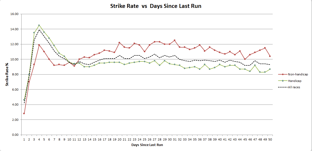
We can see that the quick turnaround Strike Rate peak is most pronounced in handicaps. But for non-handicaps the notable feature is really a lowering of Strike Rate in the 7-14 day range. It’s also interesting to see that handicaps generally have a lower Strike Rate than non-handicaps, perhaps due to field size trends. And as you would expect, running within one or two days of a prior run is rarely a good idea !
But there’s an even better way to structure a query to return the data for all races, handicaps and non-handicaps by adding the handicap field to both SELECT clauses and the GROUP BY with a ROLLUP for good measure:
SELECT
    sub.days_since_ran,
    sub.handicap,
    sub.race_count,
    sub.win_count,
    round(sub.win_count / sub.race_count * 100, 1) AS strike_rate
FROM (
    SELECT
        days_since_ran,
        handicap,
        COUNT(*) as race_count,
        COUNT(IF(finish_position = 1, 1, NULL)) AS win_count
    FROM
        historic_runners_beta
    JOIN
        historic_races_beta
    USING(race_id)
    WHERE
        days_since_ran IS NOT NULL AND
        year(meeting_date) >= 2010
    GROUP BY days_since_ran, handicap WITH ROLLUP
    ORDER BY days_since_ran, handicap LIMIT 150) AS sub;
The first 15 lines of the resulting table looks like this:
+----------------+----------+------------+-----------+-------------+
| days_since_ran | handicap | race_count | win_count | strike_rate |
+----------------+----------+------------+-----------+-------------+
|           NULL |     NULL |    1496886 |    145734 |         9.7 |
|              1 |     NULL |       5051 |       210 |         4.2 |
|              1 |        0 |       1292 |        36 |         2.8 |
|              1 |        1 |       3759 |       174 |         4.6 |
|              2 |     NULL |       7250 |       566 |         7.8 |
|              2 |        0 |       1580 |       110 |         7.0 |
|              2 |        1 |       5670 |       456 |         8.0 |
|              3 |     NULL |       7839 |       988 |        12.6 |
|              3 |        0 |       1671 |       155 |         9.3 |
|              3 |        1 |       6168 |       833 |        13.5 |
|              4 |     NULL |      10054 |      1397 |        13.9 |
|              4 |        0 |       2300 |       274 |        11.9 |
|              4 |        1 |       7754 |      1123 |        14.5 |
|              5 |     NULL |      13140 |      1705 |        13.0 |
|              5 |        0 |       3101 |       341 |        11.0 |
|              5 |        1 |      10039 |      1364 |        13.6 |
where the rows with handicap = NULL represent the All Races data. While this is less convenient for importing into Excel to make a chart, it is closer to what you may want as a data mapping table for normalizing data to be passed onto a ML system. The top double NULL row gives the Strike Rate for all runners in all races of all types irrespective of days_since_ran as 9.7% – a useful baseline number.
A question for the reader. If the average Strike Rate for all runners in all races of all types is 9.7%, can you use that information to calculate the average number of runners per race ? And what simple one liner query would you use to check your result ? Answers in the comments please 🙂
The final point to tie up is what if you want to use this as a days_since_ran to Strike Rate conversion so that you can present normalized data to your downstream ML system. The simplest solution is to store this data back into the database as a data mapping table by prefixing the outer SELECT with:
DROP TABLE IF EXISTS days_since_ran_x_strike_rate;
CREATE TABLE days_since_ran_x_strike_rate(
    days_since_ran   int(4),
    handicap         tinyint(1),
    race_count       int(6),
    win_count        int(6),
    strike_rate      decimal(4,1));
INSERT INTO days_since_ran_x_strike_rate
SELECT
   ...
You can then use this data mapping table for days_since_ran to Strike Rate conversion by performing a JOIN as follows (incomplete code):
SELECT
    strike_rate
FROM
    daily_runners
JOIN
    days_since_ran_x_strike_rate
USING(days_since_ran)
To make this work reliably is a little more complex because once over 50 days you need to bucket day ranges or perhaps have a single bucket for > 50 with the LIMIT 50 removed, which in turn means working CASE into your SQL.
For automation, you can set the whole thing up as a stored procedure which you run daily as a Windows scheduled job or Linux cron job, shortly after your daily database update.