
Calculating Profit and Loss from Historic Data using R
By Phill Clarke on Saturday, May 19th, 2018Previously we looked at how to calculate the strike rate for jockeys, specifically with relation to those riding in the 1000 Guineas. The result of that race showed how strikes rates are really only part of the overall picture. Sean Levey had the lowest historic strike rate for Group races, of all those peforming in the 1000 Guineas, yet rode a convincing winner. If we had of looked at trainer strike rates, it may have been a different story.
This article will now look at trainer strike rates, but also specifically calculate the profit and loss (P&L) to show what would happen if one had backed every runner for a specific trainer at starting price (SP) in all Group races.
We start very similar to previously, returning historic data from the Smartform database and calculating trainer strike rates.
# Load the RMySQL and dplyr library packages
library("RMySQL")
library("dplyr")

# Execute an SQL command to return some historic data
# Connect to the Smartform database. Substitute the placeholder credentials for your own.
# The IP address can be substituted for a remote location if appropriate.
con <- dbConnect(MySQL(),
                        host='127.0.0.1',
                        user='yourusername',
                        password='yourpassword',
                        dbname='smartform')

# This SQL query selects the required columns from the historic_races and historic_runners tables, joining by unique race_id and filtering for results only since January 1st, 2006. The SQL query is saved in a variable called sql1.
sql1 <- paste("SELECT historic_races.course,
              historic_races.meeting_date,
              historic_races.conditions,
              historic_races.group_race,
              historic_races.race_type_id,
              historic_races.race_type,
              historic_runners.name,
              historic_runners.jockey_name,
              historic_runners.trainer_name,
              historic_runners.finish_position,
              historic_runners.starting_price_decimal
              FROM smartform.historic_runners
              JOIN smartform.historic_races USING (race_id)
              WHERE historic_races.meeting_date >= '2006-01-01'", sep="")

# Now execute the SQL query, using the previously established connection. Results are stored in a variable called smartform_results.
smartform_results <- dbGetQuery(con, sql1)

# Close the database connection, which is good practice
dbDisconnect(con)

# Race type IDs 12 and 15 correspond to Flat and All Weather races
flat_races_only <- dplyr::filter(smartform_results,
                                  race_type_id == 12 |
                                   race_type_id == 15)

# Filter using the group_race field for Group 1, 2 and 3 races only
group_races_only <- dplyr::filter(flat_races_only,
                                group_race == 1 |
                                  group_race == 2 |
                                  group_race == 3 )

# For each trainer name, count the number of runs
trainer_group_runs <- group_races_only %>% count(trainer_name)

# Rename the second column in trainer_group_rides to something more logical
names(trainer_group_runs)[2]<-"group_runs"

# Now filter for only winning runs
group_winners_only <- dplyr::filter(group_races_only,
                                    finish_position == 1)

# For each trainer, count the number of winning runs
trainer_group_wins <- group_winners_only %>% count(trainer_name)

# Rename the second column in trainer_group_wins to something more logical
names(trainer_group_wins)[2]<-"group_wins"

# Join the two dataframes, trainer_group_runs and trainer_group_wins together, using trainer_name as a key
trainer_group_data <- dplyr::full_join(trainer_group_runs, trainer_group_wins, by = "trainer_name")


# Rename all the NA fields in the new dataframe to zero
# If a trainer has not had a group winner, the group_wins field will be NA
# If this is not changed to zero, later calculations will fail
trainer_group_data[is.na(trainer_group_data)] <- 0

# Now calculate the Group race strike rate for all trainers
trainer_group_data$strike_rate <- (trainer_group_data$group_wins / trainer_group_data$group_runs) * 100
The variable trainer_group_data now contains the strike rate for every trainer who has had a runner in a flat or all weather Group race since January 1st, 2006.
The Group 1 Lockinge Stakes is run today at Newbury. Therefore, let’s look at this field only for today’s examples.
# Execute an SQL command to return some daily data
# Connect to the Smartform database. Substitute the placeholder credentials for your own.
# The IP address can be substituted for a remote location if appropriate.
con <- dbConnect(MySQL(),
                        host='127.0.0.1',
                        user='yourusername',
                        password='yourpassword',
                        dbname='smartform')

# This SQL query selects the required columns from the daily_races and daily_runners tables, joining by unique race_id and filtering for results only with today's date. The SQL query is saved in a variable called sql2.
sql2 <- paste("SELECT daily_races.course,
              daily_races.race_title,
              daily_races.meeting_date,
              daily_runners.name,
              daily_runners.jockey_name,
              daily_runners.trainer_name
              FROM smartform.daily_races
              JOIN smartform.daily_runners USING (race_id)
              WHERE daily_races.meeting_date >='2018-05-18'", sep="")

# Now execute the SQL query, using the previously established connection. Results are stored in a variable called smartform_daily_results.
smartform_daily_results <- dbGetQuery(con, sql2)

# Close the database connection, which is good practice
dbDisconnect(con)
The variable smartform_daily_results contains information about all races being run today.
Now we filter for just today’s Lockinge Stakes.
# Filter for the Lockinge Stakes only
lockinge_only <- dplyr::filter(smartform_daily_results,
                              grepl("Lockinge", race_title))
The variable lockinge_only now contains just the basic details for today’s Group 1 Lockinge Stakes.
Lastly, dplyr is again used to perform a different type of join, which combines the lockinge_only and trainer_group_data dataframes, using trainer_name as the key.
# Using dplyr, join the lockinge_only and trainer_group_data dataframes
lockinge_only_with_sr <- dplyr::inner_join(lockinge_only, trainer_group_data, by = "trainer_name")
If we now view the dataframe lockinge_only_with_sr we can see that the trainer with the best strike rate in Group races, with runners also in today’s Lockinge Stakes, is Aiden O’Brien.
lockinge_only_with_sr

    course                                race_title meeting_date             name    jockey_name         trainer_name group_rides group_wins strike_rate
1  Newbury Al Shaqab Lockinge Stakes (Group 1) (Str)   2018-05-19  Lightning Spear   Oisin Murphy          D M Simcock         256         24    9.375000
2  Newbury Al Shaqab Lockinge Stakes (Group 1) (Str)   2018-05-19          Suedois      D Tudhope            D O'Meara         190         16    8.421053
3  Newbury Al Shaqab Lockinge Stakes (Group 1) (Str)   2018-05-19           Limato  Harry Bentley              H Candy         103         15   14.563107
4  Newbury Al Shaqab Lockinge Stakes (Group 1) (Str)   2018-05-19   Librisa Breeze      R Winston            D K Ivory          44          2    4.545455
5  Newbury Al Shaqab Lockinge Stakes (Group 1) (Str)   2018-05-19       Zonderland        A Kirby              C G Cox         265         30   11.320755
6  Newbury Al Shaqab Lockinge Stakes (Group 1) (Str)   2018-05-19        Deauville     W M Lordan          A P O'Brien        2347        385   16.403920
7  Newbury Al Shaqab Lockinge Stakes (Group 1) (Str)   2018-05-19 Accidental Agent Charles Bishop Eve Johnson Houghton          70          1    1.428571
8  Newbury Al Shaqab Lockinge Stakes (Group 1) (Str)   2018-05-19 Lancaster Bomber  J A Heffernan          A P O'Brien        2347        385   16.403920
9  Newbury Al Shaqab Lockinge Stakes (Group 1) (Str)   2018-05-19    Beat The Bank    Jim Crowley          A M Balding         367         25    6.811989
10 Newbury Al Shaqab Lockinge Stakes (Group 1) (Str)   2018-05-19       War Decree      P B Beggy          A P O'Brien        2347        385   16.403920
11 Newbury Al Shaqab Lockinge Stakes (Group 1) (Str)   2018-05-19     Rhododendron      R L Moore          A P O'Brien        2347        385   16.403920
12 Newbury Al Shaqab Lockinge Stakes (Group 1) (Str)   2018-05-19 Alexios Komnenos      C D Hayes            J A Stack          19          3   15.789474
13 Newbury Al Shaqab Lockinge Stakes (Group 1) (Str)   2018-05-19           Lahore     S De Sousa              C G Cox         265         30   11.320755
14 Newbury Al Shaqab Lockinge Stakes (Group 1) (Str)   2018-05-19          Addeybb    James Doyle           W J Haggas         459         48   10.457516
No real suprises there perhaps. However, what would now happen if we’d placed a one Pound bet on every Aiden O’Brien runner in Group races over the last twelve years. Would we have made a profit?
To begin, we filter all historic Group races, from the data obtained earlier, for just Aiden O’Brien’s horses.
# Filter historic data just for A P O'Brien horses
obrien_group_races_only <- dplyr::filter(group_races_only,
                                         grepl("A P O'Brien", trainer_name))

# Non Runners appears as NA, which need to be removed for a true picture and so calulations do not fail
obrien_group_races_only <- dplyr::filter(obrien_group_races_only, !is.na(finish_position))
The dataframe obrien_group_races_only now contains the data we need.
The next step is to cumulatively sum all the start prices for winning horses and deduct our one Pound stake where appropriate. The cumsum function is used to achieve this. The ifelse statement below basically says, for all lines in the dataframe where the finishing position is one, use the decimal starting price but also subtract our initial one Pound stake, otherwise (if the finish position isn’t one) simply subtract our one Pound stake from the total.
# Calculate the cumulative total for all O'Brien runners
obrien_cumulative <- cumsum(
  ifelse(obrien_group_races_only$finish_position == 1, (obrien_group_races_only$starting_price_decimal-1),-1)
)

# Add a new column back into obrien_group_races_only, with the cumulative totals
obrien_group_races_only$cumulative <- obrien_cumulative
When viewing the dataframe obrien_group_races_only you will now see a new column included called cumulative. Looking at the last entry for this column in the dataframe, the results is -275.76. Therefore, a single Pound bet on all 2178 Aiden O’Brien Group race runners since 2006 would have resulted in a loss of £275.76. Not really the route to profitable punting.
We can also take this a step further and plot the results for something more visual. The code below uses the gglot2 library again, along with some helper libraries in order to make a prettier chart.
# Load relevant libraries
library("ggplot2")
library("ggthemes")
library("scales")

# Convert the meeting_date column from character format to Date format
obrien_group_races_only$meeting_date <- as.Date(obrien_group_races_only$meeting_date)

# Plot the chart
ggplot(data=obrien_group_races_only, aes(x=meeting_date, y=cumulative, group=1)) +
  geom_line(colour="blue", lwd=0.7) +
  scale_x_date(labels = date_format("%Y-%m-%d"), date_breaks="6 months") +
  scale_y_continuous(breaks = seq(-300, 10, by = 50)) +
  theme_tufte(base_family="serif", base_size = 14) +
  geom_rangeframe() +
  theme(axis.text.x = element_text(angle = 45, hjust = 1),
        panel.grid.major.x = element_line(color = "grey80"),
        panel.grid.major.y = element_line(color = "grey80"))
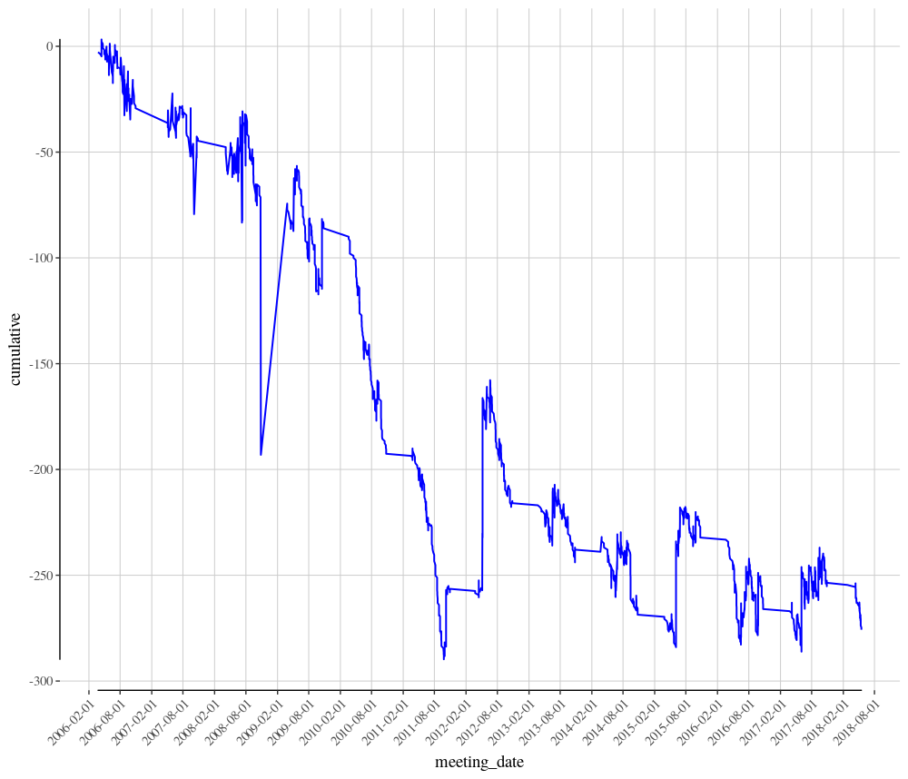
The years 2009 through to the end of 2011 look to be particularly poor years for Aiden O’Brien in Group races, but 2014 onwards has been much more stable.
Today we have shown that just because the trainer may have the best historic strike rate in Group races, backing all of their runners blindly does not necessarily result in a profit. The market obviously knows the A P O’Brien has a very good record in these types of races and his horses are priced accordingly.
An exercise for the reader could be to calculate the P&L for Aiden O’Brien runners when ridden by Ryan Moore. To do this, start by filtering the historic obrien_group_races_only data by R L Moore. Hint: The answer is they are an profitable combination over 375 runs since 2006.
Questions and queries about this article should be posted as a comment below or to the Betwise Q&A board.
The full R code used in this article is found below.
# Load the RMySQL and dplyr library packages
library("RMySQL")
library("dplyr")

# Execute an SQL command to return some historic data
# Connect to the Smartform database. Substitute the placeholder credentials for your own.
# The IP address can be substituted for a remote location if appropriate.
con <- dbConnect(MySQL(),
                        host='127.0.0.1',
                        user='yourusername',
                        password='yourpassword',
                        dbname='smartform')

# This SQL query selects the required columns from the historic_races and historic_runners tables, joining by unique race_id and filtering for results only since January 1st, 2006. The SQL query is saved in a variable called sql1.
sql1 <- paste("SELECT historic_races.course,
              historic_races.meeting_date,
              historic_races.conditions,
              historic_races.group_race,
              historic_races.race_type_id,
              historic_races.race_type,
              historic_runners.name,
              historic_runners.jockey_name,
              historic_runners.trainer_name,
              historic_runners.finish_position,
              historic_runners.starting_price_decimal
              FROM smartform.historic_runners
              JOIN smartform.historic_races USING (race_id)
              WHERE historic_races.meeting_date >= '2006-01-01'", sep="")

# Now execute the SQL query, using the previously established connection. Results are stored in a variable called smartform_results.
smartform_results <- dbGetQuery(con, sql1)

# Close the database connection, which is good practice
dbDisconnect(con)

# Race type IDs 12 and 15 correspond to Flat and All Weather races
flat_races_only <- dplyr::filter(smartform_results,
                                  race_type_id == 12 |
                                   race_type_id == 15)

# Filter using the group_race field for Group 1, 2 and 3 races only
group_races_only <- dplyr::filter(flat_races_only,
                                group_race == 1 |
                                  group_race == 2 |
                                  group_race == 3 )

# For each trainer name, count the number of runs
trainer_group_runs % count(trainer_name)

# Rename the second column in trainer_group_rides to something more logical
names(trainer_group_runs)[2]<-"group_runs"

# Now filter for only winning runs
group_winners_only <- dplyr::filter(group_races_only,
                                    finish_position == 1)

# For each trainer, count the number of winning runs
trainer_group_wins % count(trainer_name)

# Rename the second column in trainer_group_wins to something more logical
names(trainer_group_wins)[2]<-"group_wins"

# Join the two dataframes, trainer_group_runs and trainer_group_wins together, using trainer_name as a key
trainer_group_data <- dplyr::full_join(trainer_group_runs, trainer_group_wins, by = "trainer_name")


# Rename all the NA fields in the new dataframe to zero
# If a trainer has not had a group winner, the group_wins field will be NA
# If this is not changed to zero, later calculations will fail
trainer_group_data[is.na(trainer_group_data)] <- 0

# Now calculate the Group race strike rate for all trainers
trainer_group_data$strike_rate <- (trainer_group_data$group_wins / trainer_group_data$group_runs) * 100

# Execute an SQL command to return some daily data
# Connect to the Smartform database. Substitute the placeholder credentials for your own.
# The IP address can be substituted for a remote location if appropriate.
con <- dbConnect(MySQL(),
                        host='127.0.0.1',
                        user='yourusername',
                        password='yourpassword',
                        dbname='smartform')

# This SQL query selects the required columns from the daily_races and daily_runners tables, joining by unique race_id and filtering for results only with today's date. The SQL query is saved in a variable called sql2.
sql2 <- paste("SELECT daily_races.course,
              daily_races.race_title,
              daily_races.meeting_date,
              daily_runners.name,
              daily_runners.jockey_name,
              daily_runners.trainer_name
              FROM smartform.daily_races
              JOIN smartform.daily_runners USING (race_id)
              WHERE daily_races.meeting_date >='2018-05-18'", sep="")

# Now execute the SQL query, using the previously established connection. Results are stored in a variable called smartform_daily_results.
smartform_daily_results <- dbGetQuery(con, sql2)

# Close the database connection, which is good practice
dbDisconnect(con)

# Filter for the Lockinge Stakes only
lockinge_only <- dplyr::filter(smartform_daily_results,
                              grepl("Lockinge", race_title))

# Using dplyr, join the lockinge_only and trainer_group_data dataframes
lockinge_only_with_sr <- dplyr::inner_join(lockinge_only, trainer_group_data, by = "trainer_name")

# Filter historic data just for A P O'Brien horses
obrien_group_races_only <- dplyr::filter(group_races_only,
                                         grepl("A P O'Brien", trainer_name))

# Non Runners appears as NA, which need to be removed for a true picture and so calulations do not fail
obrien_group_races_only <- dplyr::filter(obrien_group_races_only, !is.na(finish_position))

# Calculate the cumulative total for all O'Brien runners
obrien_cumulative <- cumsum(
  ifelse(obrien_group_races_only$finish_position == 1, (obrien_group_races_only$starting_price_decimal-1),-1)
)

# Add a new column back into obrien_group_races_only, with the cumulative totals
obrien_group_races_only$cumulative <- obrien_cumulative

# Load relevant libraries
library("ggplot2")
library("ggthemes")
library("scales")

# Convert the meeting_date column from character format to Date format
obrien_group_races_only$meeting_date <- as.Date(obrien_group_races_only$meeting_date)

# Plot the chart
ggplot(data=obrien_group_races_only, aes(x=meeting_date, y=cumulative, group=1)) +
  geom_line(colour="blue", lwd=0.7) +
  scale_x_date(labels = date_format("%Y-%m-%d"), date_breaks="6 months") +
  scale_y_continuous(breaks = seq(-300, 10, by = 50)) +
  theme_tufte(base_family="serif", base_size = 14) +
  geom_rangeframe() +
  theme(axis.text.x = element_text(angle = 45, hjust = 1),
        panel.grid.major.x = element_line(color = "grey80"),
        panel.grid.major.y = element_line(color = "grey80"))

##################################################################################
# Reader Exercise: Aiden O'Brien and Ryan Moore combined in Group Races
##################################################################################

obrien_moore_group_races_only <- dplyr::filter(obrien_group_races_only,
                                               grepl("R L Moore", jockey_name))

obrien_moore_cumulative <- cumsum(
  ifelse(obrien_moore_group_races_only$finish_position == 1, (obrien_moore_group_races_only$starting_price_decimal-1),-1)
)

obrien_moore_group_races_only$cumulative <- obrien_moore_cumulative


obrien_moore_group_races_only$meeting_date <- as.Date(obrien_moore_group_races_only$meeting_date)


ggplot(data=obrien_moore_group_races_only, aes(x=meeting_date, y=cumulative, group=1)) +
  geom_line(colour="blue", lwd=0.7) +
  scale_x_date(labels = date_format("%Y-%m-%d"), date_breaks="6 months") +
  theme_tufte(base_family="serif", base_size = 14) +
  geom_rangeframe() +
  theme(axis.text.x = element_text(angle = 45, hjust = 1),
        panel.grid.major.x = element_line(color = "grey80"),
        panel.grid.major.y = element_line(color = "grey80"))