
Archive for June, 2018
Plotting Trainer, Jockey and Sire Statistics in a Stacked Bar Chart with R
Saturday, June 23rd, 2018Earlier in the week we looked at how to use a for loop to iterate across rows of a dataframe to calculate statistics in an automated manner. Interesting and useful, but we only looked at one specific set of circumstance; trainer and jockey combinations in Group races. There are many other useful statistics which can be used to examine a race. This article focuses on today’s Diamond Jubilee Stakes at Royal Ascot, extends the one collection of statistics to four and finally plots the outcome in a visual format.
As the code examples for this article now extend to beyond 550 lines, it is not practicle to include all the code in-line with the article text. Therefore, only certain examples will be included in-line with the full R code will be provided at the end of the article.
The initial assumption is that data has been returned from the Smartform database, although some additional field are now returned, specifically trainer_id, jockey_id and sire_name.
# Select relevant historic results
sql1 <- paste("SELECT historic_races.course,
              historic_races.meeting_date,
              historic_races.conditions,
              historic_races.group_race,
              historic_races.race_type_id,
              historic_races.race_type,
              historic_races.distance_yards,
              historic_runners.name,
              historic_runners.jockey_name,
              historic_runners.trainer_name,
              historic_runners.finish_position,
              historic_runners.starting_price_decimal,
              historic_runners.trainer_id,
              historic_runners.jockey_id,
              historic_runners.sire_name
              FROM smartform.historic_runners
              JOIN smartform.historic_races USING (race_id)
              WHERE historic_races.meeting_date >= '2012-01-01'", sep="")
Previously we created a trainer & jockey function to investigate these specific combinations in Group races. This is now extended to just trainer, just jockey and just sire functions. The trainer function is found below.
# Trainer stats
# Name the function and add some arguments
tr <- function(race_filter = "", price_filter = 1000, trainer){

  # Filter for flat races only
  flat_races_only <- dplyr::filter(smartform_results,
                                   race_type_id == 12 |
                                     race_type_id == 15)

  # Add an if else statement for the race_filter argument
  if (race_filter == "group"){

    filtered_races <- dplyr::filter(flat_races_only,
                                    group_race == 1 |
                                      group_race == 2 |
                                      group_race == 3 )
  } else {

    filtered_races = flat_races_only
  }

  # Filter by trainer id
  trainer_filtered <- dplyr::filter(filtered_races,
                                    grepl(trainer, trainer_id))


  # Filter by price
  trainer_price_filtered <- dplyr::filter(trainer_filtered,
                                                 starting_price_decimal <= price_filter)

  #  Calculate Profit and Loss
  trainer_cumulative <- cumsum(
    ifelse(trainer_price_filtered$finish_position == 1,
           (trainer_price_filtered$starting_price_decimal-1),
           -1)
  )

  # Calculate Strike Rate
  winners <- nrow(dplyr::filter(trainer_price_filtered,
                                finish_position == 1))

  runners <- nrow(trainer_price_filtered)

  strike_rate <- (winners / runners) * 100

  # Calculate Profit on Turnover or Yield
  profit_on_turnover <- (tail(trainer_cumulative, n=1) / runners) * 100

  # Check if POT is zero length to catch later errors
  if (length(profit_on_turnover) == 0) profit_on_turnover <- 0

  # Calculate Impact Values
  # First filter all runners by price, to return those just starting at the price_filter or less
  all_runners <- nrow(dplyr::filter(filtered_races,
                                    starting_price_decimal <= price_filter))

  # Filter all winners by the price filter
  all_winners <- nrow(dplyr::filter(filtered_races,
                                    finish_position == 1 &
                                      starting_price_decimal <= price_filter))

  # Now calculate the Impact Value
  iv <- (winners / all_winners) / (runners / all_runners)

  # Calculate Actual vs Expected ratio
  # # Convert all decimal odds to probabilities
  total_sp <- sum(1/trainer_price_filtered$starting_price_decimal)

  # Calculate A/E by dividing the number of  winners, by the sum of all SP probabilities.
  ae <- winners / total_sp

  # Calculate Archie
  archie <- (runners * (winners  - total_sp)^2)/ (total_sp  * (runners - total_sp))

  # Calculate the Confidence figure
  conf <- pchisq(archie, df = 1)*100

  # Create an empty variable
  trainer <- NULL

  # Add all calculated figures as named objects to the variable, which creates a list
  trainer$tr_runners <- runners
  trainer$tr_winners <- winners
  trainer$tr_sr <- strike_rate
  trainer$tr_pot <- profit_on_turnover
  trainer$tr_iv <- iv
  trainer$tr_ae <- ae
  trainer$tr_conf <- conf

  # Add an error check to convert all NaN values to zero
  final_results <- unlist(trainer)
  final_results[ is.nan(final_results) ] <- 0

  # Manipulate the layout of returned results to be a nice dataframe
  final_results <- t(as.data.frame(final_results))
  rownames(final_results) <- c()

  # 2 decimal places only
  round(final_results, 2)

  # Finally, close the function
}
Note that in the above code, instead of filtering by trainer_name, we are now filtering by trainer_id. This is due to the fact that sometimes the trainer names in the daily racing data do not exactly match those in the historic data. For example, Sir Michael Stoute hasn’t always been a knight. Therefore, if we were just matching on trainer_name there would be some occassions where this fails and no results are returned. Smartform instead provides a unique identification number for trainers and jockeys, which insures there will always be a match between historic and daily data.
The function above is just one example. In order to produce the charts later in this article, additional jockey and sire functions have been added, bringing the total to four; trainer, jockey, trainer & jockey and sire. The number of statistics could be extended much further to include angles such as trainer & distance, trainer & course, trainer & age (2yo, 3yo, 4yo+ races) and many more.
The for loop also now includes all four of these functions.
# Create placeholder lists which will be required later
row_tr <- list()
row_jc <- list()
row_tj <- list()
row_sr <- list()

# Setup the loop
# For each horse in the group_races_only dataframe
for (i in group_races_only$name) {


  runner_details = group_races_only[group_races_only$name==i,]

  # Extract trainer, jockey id and sire names
  trainer <- runner_details$trainer_id
  jockey <- runner_details$jockey_id
  sire <- runner_details$sire_name

  # Apply the Trainer function for Group races only
  trainer_combo <- tr(race_filter = "group",
                                  trainer = trainer)

  # Add results row by row to the previously defined list
  row_tr[[i]] <- trainer_combo

  # Apply the Jockey function for Group races only
  jockey_combo <- jc(race_filter = "group",
                             jockey = jockey)

  # Add results row by row to the previously defined list
  row_jc[[i]] <- jockey_combo

  # Apply the Trainer/Jockey function for Group races only
  trainer_jockey_combo <- tj(race_filter = "group",
                             trainer = trainer, jockey = jockey)

  # Add results row by row to the previously defined list
  row_tj[[i]] <- trainer_jockey_combo

  # Apply the Sire function for Group races only
  sire_combo <- sr(race_filter = "group",
                             sire = sire)

  # Add results row by row to the previously defined list
  row_sr[[i]] <- sire_combo

  # Create a final dataframe
  stats_final_tr <- as.data.frame(do.call("rbind", row_tr))
  stats_final_jc <- as.data.frame(do.call("rbind", row_jc))
  stats_final_tj <- as.data.frame(do.call("rbind", row_tj))
  stats_final_sr <- as.data.frame(do.call("rbind", row_sr))

}

# Create a new variable called racecard. Bind together the generic race details with the newly created stats
racecard <- cbind(group_races_only,stats_final_tr)
racecard <- cbind(racecard,stats_final_jc)
racecard <- cbind(racecard,stats_final_tj)
racecard <- cbind(racecard,stats_final_sr)
Viewing the final racecard now shows forty columns and a wall of data. This isn’t perhaps the easiest way to visualise the overall picture. Instead, we’ll create a stacked barchart showing Impact Values for all four angles. The legend shows tr_iv, jc_iv, tj_iv and sr_iv for the trainer, jockey, trainer & jockey and sire impact values.
# Filter for Diamond Jubilee Only
diamond_jubilee <- dplyr::filter(racecard,
                                 grepl("Diamond Jubilee",
                                       race_title))

# Filter for just the IV columns which we will plot
racecard_filtered_iv <- diamond_jubilee[,c("name","tr_iv","jc_iv", "tj_iv", "sr_iv")]

# Convert the racecard from wide to long format
racecard_long_iv <- melt(racecard_filtered_iv, id.var="name")

# Plot a stacked barchart
ggplot(racecard_long_iv, aes(x = name, y = value, fill = variable)) +
  geom_bar(stat = "identity") +
  theme(axis.text.x = element_text(angle = 45, hjust = 1))
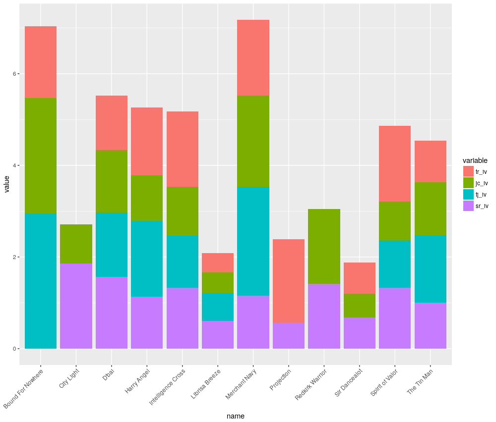
The highest bars indicate the highest cumulative Impact Values. Some bars do not include all four factors, as sometimes there were no results returned. For example, Bound For Nowhere’s sire, The Factor, has only had one Group runner in the UK & Ireland, which did not win. Therefore, there is no data to calculate strike rate, impact value etc.
This means one needs to be careful examining the chart and also take time to ponder the data in the dataframe. Some sample sizes may be very small and a question should be asked if they are statistically relevant. Bound For Nowhere’s Trainer & Jockey Impact Value is the highest in the race, but this is from only six runners. Compared to Merchant Navy with the second highest tj_iv, but from 357 runners.
Nonetheless, a visual method like this can still assist to narrow the field. Harry Angel, the favourite for the race, is certainly not a standout in the chart, with decent sample sizes across all four factors.
The stacked barchart can also be applied to Actual vs Expected figures, strike rates or Confidence figures. The chart below displays stacked A/E for a more value oriented view.
# Filter for just the AE columns which we will plot
racecard_filtered_ae <- diamond_jubilee[,c("name","tr_ae","jc_ae", "tj_ae", "sr_ae")]

# Convert the racecard from wide to long format
racecard_long_ae <- melt(racecard_filtered_ae, id.var="name")

# Plot a stacked barchart
ggplot(racecard_long_ae, aes(x = name, y = value, fill = variable)) +
  geom_bar(stat = "identity") +
  theme(axis.text.x = element_text(angle = 45, hjust = 1))
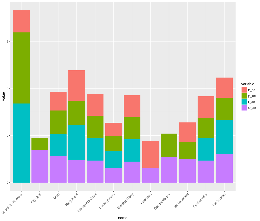
Once again, keep Bound for Nowhere’s small sample sizes in mind. Harry Angel appears to be a better betting proposition based on this chart.
Another way to look at this data might be as a grouped bar chart, where the IV and A/E figures are plotted for each horse next to each other.
# Filter for just the AE columns which we will plot
racecard_filtered_all <- diamond_jubilee[,c("name","tr_iv","jc_iv", "tj_iv", "sr_iv",
                                            "tr_ae","jc_ae", "tj_ae", "sr_ae")]

# Convert the racecard from wide to long format
racecard_long_all <- melt(racecard_filtered_all, id.var="name")

# Plot a grouped barchart
ggplot(racecard_long_all, aes(x = name, y = value, fill = variable)) +
  geom_bar(position = "dodge", stat="identity") +
  theme(axis.text.x = element_text(angle = 45, hjust = 1))
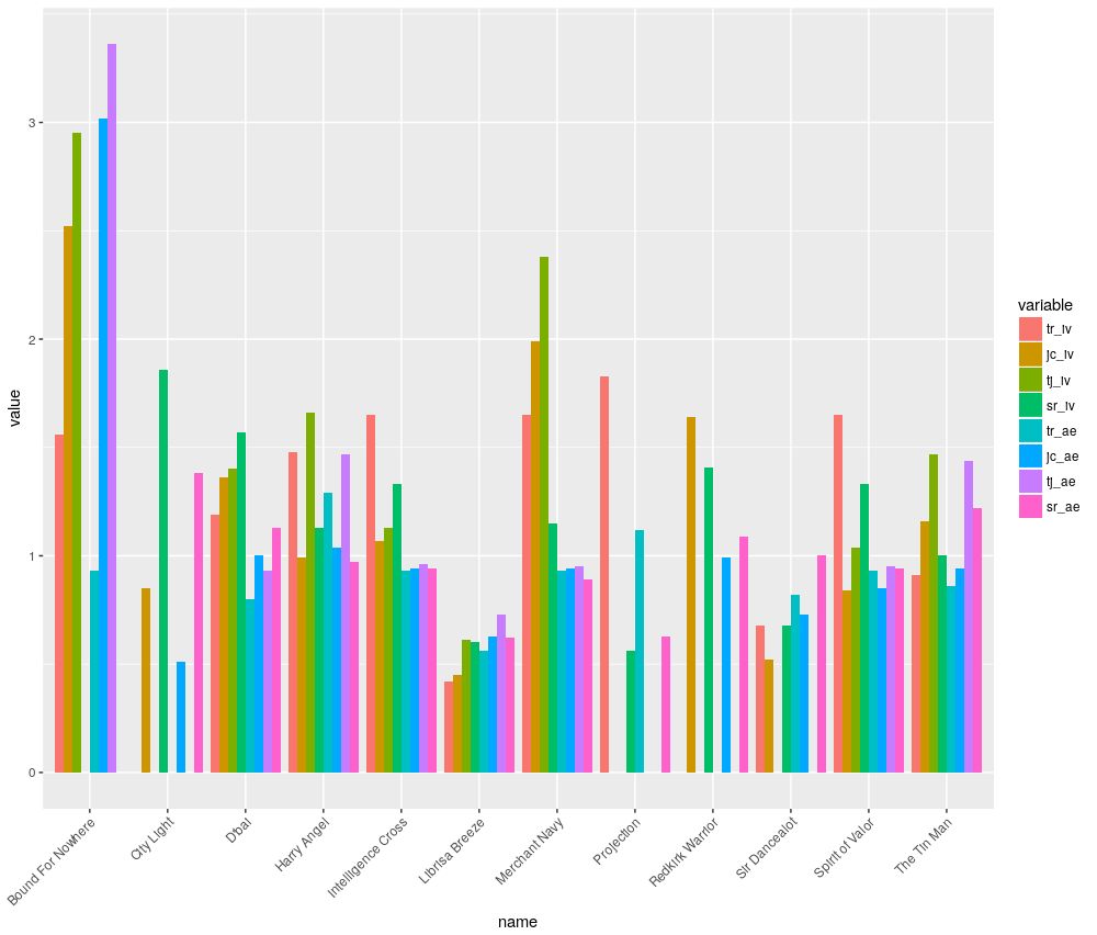
Although Sire IV is missing for Bound for Nowhere, his other figures do all point to a superier trainer and jockey, albeit from small sample size. How to statistically deal with these small sample sizes will be covered in a future article on Bayesian techniques.
Which horses might be included in a shortlist for today’s Diamond Jubilee? Even with small sample sizes, but knowing Wesley Ward’s Ascot success with sprinters, it may be wise to include Bound for Nowhere, who is currently 14.0 on Betfair. Merchant Navy (IV) and Harry Angel (A/E) are both positives, although much shorter priced at the top of the market.
It is important not to just rely on the data. There are many different factors to consider and a good knowledge of general form is also required. Therefore, after all that work, one might still decide just to back the Aussie danger and triple Group 1 sprint winner, Redkirk Warrior.
Good luck!
Questions and queries about this article should be posted as a comment below or on the Betwise Q&A board.
The full R code used in this article is found below.
# Load the library packages
library("RMySQL")
library("dplyr")
library("reshape2")
library("ggplot2")

# Connect to the Smartform database. Substitute the placeholder credentials for your own.
# The IP address can be substituted for a remote location if appropriate.
con <- dbConnect(MySQL(),
                 host='127.0.0.1',
                 user='yourusername',
                 password='yourpassword',
                 dbname='smartform')

# Select relevant historic results
sql1 <- paste("SELECT historic_races.course,
              historic_races.meeting_date,
              historic_races.conditions,
              historic_races.group_race,
              historic_races.race_type_id,
              historic_races.race_type,
              historic_races.distance_yards,
              historic_runners.name,
              historic_runners.jockey_name,
              historic_runners.trainer_name,
              historic_runners.finish_position,
              historic_runners.starting_price_decimal,
              historic_runners.trainer_id,
              historic_runners.jockey_id,
              historic_runners.sire_name
              FROM smartform.historic_runners
              JOIN smartform.historic_races USING (race_id)
              WHERE historic_races.meeting_date >= '2012-01-01'", sep="")

smartform_results <- dbGetQuery(con, sql1)

# Remove non-runners and non-finishers
smartform_results <- dplyr::filter(smartform_results, !is.na(finish_position))

# Select relevant daily results for tomorrow
sql2 <- paste("SELECT daily_races.course,
              daily_races.race_title,
              daily_races.meeting_date,
              daily_races.distance_yards,
              daily_runners.cloth_number,
              daily_runners.name,
              daily_runners.trainer_name,
              daily_runners.jockey_name,
              daily_runners.sire_name,
              daily_runners.forecast_price_decimal,
              daily_runners.trainer_id,
              daily_runners.jockey_id
              FROM smartform.daily_races
              JOIN smartform.daily_runners USING (race_id)
              WHERE daily_races.meeting_date >='2018-06-23'", sep="")

smartform_daily_results <- dbGetQuery(con, sql2)

dbDisconnect(con)

# Remove non-runners
smartform_daily_results <- dplyr::filter(smartform_daily_results, !is.na(forecast_price_decimal))

# Trainer stats
# Name the function and add some arguments
tr <- function(race_filter = "", price_filter = 1000, trainer){

  # Filter for flat races only
  flat_races_only <- dplyr::filter(smartform_results,
                                   race_type_id == 12 |
                                     race_type_id == 15)

  # Add an if else statement for the race_filter argument
  if (race_filter == "group"){

    filtered_races <- dplyr::filter(flat_races_only,
                                    group_race == 1 |
                                      group_race == 2 |
                                      group_race == 3 )
  } else {

    filtered_races = flat_races_only
  }

  # Filter by trainer name
  trainer_filtered <- dplyr::filter(filtered_races,
                                    grepl(trainer, trainer_id))


  # Filter by price
  trainer_price_filtered <- dplyr::filter(trainer_filtered,
                                                 starting_price_decimal <= price_filter)

  #  Calculate Profit and Loss
  trainer_cumulative <- cumsum(
    ifelse(trainer_price_filtered$finish_position == 1,
           (trainer_price_filtered$starting_price_decimal-1),
           -1)
  )

  # Calculate Strike Rate
  winners <- nrow(dplyr::filter(trainer_price_filtered,
                                finish_position == 1))

  runners <- nrow(trainer_price_filtered)

  strike_rate <- (winners / runners) * 100

  # Calculate Profit on Turnover or Yield
  profit_on_turnover <- (tail(trainer_cumulative, n=1) / runners) * 100

  # Check if POT is zero length to catch later errors
  if (length(profit_on_turnover) == 0) profit_on_turnover <- 0

  # Calculate Impact Values
  # First filter all runners by price, to return those just starting at the price_filter or less
  all_runners <- nrow(dplyr::filter(filtered_races,
                                    starting_price_decimal <= price_filter))

  # Filter all winners by the price filter
  all_winners <- nrow(dplyr::filter(filtered_races,
                                    finish_position == 1 &
                                      starting_price_decimal <= price_filter))

  # Now calculate the Impact Value
  iv <- (winners / all_winners) / (runners / all_runners)

  # Calculate Actual vs Expected ratio
  # # Convert all decimal odds to probabilities
  total_sp <- sum(1/trainer_price_filtered$starting_price_decimal)

  # Calculate A/E by dividing the number of  winners, by the sum of all SP probabilities.
  ae <- winners / total_sp

  # Calculate Archie
  archie <- (runners * (winners  - total_sp)^2)/ (total_sp  * (runners - total_sp))

  # Calculate the Confidence figure
  conf <- pchisq(archie, df = 1)*100

  # Create an empty variable
  trainer <- NULL

  # Add all calculated figures as named objects to the variable, which creates a list
  trainer$tr_runners <- runners
  trainer$tr_winners <- winners
  trainer$tr_sr <- strike_rate
  trainer$tr_pot <- profit_on_turnover
  trainer$tr_iv <- iv
  trainer$tr_ae <- ae
  trainer$tr_conf <- conf

  # Add an error check to convert all NaN values to zero
  final_results <- unlist(trainer)
  final_results[ is.nan(final_results) ] <- 0

  # Manipulate the layout of returned results to be a nice dataframe
  final_results <- t(as.data.frame(final_results))
  rownames(final_results) <- c()

  # 2 decimal places only
  round(final_results, 2)

  # Finally, close the function
}

# Jockey stats
# Name the function and add some arguments
jc <- function(race_filter = "", price_filter = 1000, jockey){

  # Filter for flat races only
  flat_races_only <- dplyr::filter(smartform_results,
                                   race_type_id == 12 |
                                     race_type_id == 15)

  # Add an if else statement for the race_filter argument
  if (race_filter == "group"){

    filtered_races <- dplyr::filter(flat_races_only,
                                    group_race == 1 |
                                      group_race == 2 |
                                      group_race == 3 )
  } else {

    filtered_races = flat_races_only
  }

  # Filter by trainer name
  jockey_filtered <- dplyr::filter(filtered_races,
                                    grepl(jockey, jockey_id))


  # Filter by price
  jockey_price_filtered <- dplyr::filter(jockey_filtered,
                                          starting_price_decimal <= price_filter)

  #  Calculate Profit and Loss
  jockey_cumulative <- cumsum(
    ifelse(jockey_price_filtered$finish_position == 1,
           (jockey_price_filtered$starting_price_decimal-1),
           -1)
  )

  # Calculate Strike Rate
  winners <- nrow(dplyr::filter(jockey_price_filtered,
                                finish_position == 1))

  runners <- nrow(jockey_price_filtered)

  strike_rate <- (winners / runners) * 100

  # Calculate Profit on Turnover or Yield
  profit_on_turnover <- (tail(jockey_cumulative, n=1) / runners) * 100

  # Check if POT is zero length to catch later errors
  if (length(profit_on_turnover) == 0) profit_on_turnover <- 0

  # Calculate Impact Values
  # First filter all runners by price, to return those just starting at the price_filter or less
  all_runners <- nrow(dplyr::filter(filtered_races,
                                    starting_price_decimal <= price_filter))

  # Filter all winners by the price filter
  all_winners <- nrow(dplyr::filter(filtered_races,
                                    finish_position == 1 &
                                      starting_price_decimal <= price_filter))

  # Now calculate the Impact Value
  iv <- (winners / all_winners) / (runners / all_runners)

  # Calculate Actual vs Expected ratio
  # # Convert all decimal odds to probabilities
  total_sp <- sum(1/jockey_price_filtered$starting_price_decimal)

  # Calculate A/E by dividing the number of  winners, by the sum of all SP probabilities.
  ae <- winners / total_sp

  # Calculate Archie
  archie <- (runners * (winners  - total_sp)^2)/ (total_sp  * (runners - total_sp))

  # Calculate the Confidence figure
  conf <- pchisq(archie, df = 1)*100

  # Create an empty variable
  jockey <- NULL

  # Add all calculated figures as named objects to the variable, which creates a list
  jockey$jc_runners <- runners
  jockey$jc_winners <- winners
  jockey$jc_sr <- strike_rate
  jockey$jc_pot <- profit_on_turnover
  jockey$jc_iv <- iv
  jockey$jc_ae <- ae
  jockey$jc_conf <- conf

  # Add an error check to convert all NaN values to zero
  final_results <- unlist(jockey)
  final_results[ is.nan(final_results) ] <- 0

  # Manipulate the layout of returned results to be a nice dataframe
  final_results <- t(as.data.frame(final_results))
  rownames(final_results) <- c()

  # 2 decimal places only
  round(final_results, 2)

  # Finally, close the function
}

# Trainer and Jockey stats
# Name the function and add some arguments
tj <- function(race_filter = "", price_filter = 1000, trainer, jockey){

  # Filter for flat races only
  flat_races_only <- dplyr::filter(smartform_results,
                                   race_type_id == 12 |
                                     race_type_id == 15)

  # Add an if else statement for the race_filter argument
  if (race_filter == "group"){

    filtered_races <- dplyr::filter(flat_races_only,
                                    group_race == 1 |
                                      group_race == 2 |
                                      group_race == 3 )
  } else {

    filtered_races = flat_races_only
  }

  # Filter by trainer name
  trainer_filtered <- dplyr::filter(filtered_races,
                                    grepl(trainer, trainer_id))

  # Remove non-runners
  #  trainer_name_filtered <- dplyr::filter(trainer_filtered, !is.na(finish_position))

  # Filter by jockey name
  trainer_jockey_filtered <- dplyr::filter(trainer_filtered,
                                           grepl(jockey, jockey_id))

  # Filter by price
  trainer_jockey_price_filtered <- dplyr::filter(trainer_jockey_filtered,
                                                 starting_price_decimal <= price_filter)

  #  Calculate Profit and Loss
  trainer_jockey_cumulative <- cumsum(
    ifelse(trainer_jockey_price_filtered$finish_position == 1,
           (trainer_jockey_price_filtered$starting_price_decimal-1),
           -1)
  )

  # Calculate Strike Rate
  winners <- nrow(dplyr::filter(trainer_jockey_price_filtered,
                                finish_position == 1))

  runners <- nrow(trainer_jockey_price_filtered)

  strike_rate <- (winners / runners) * 100

  # Calculate Profit on Turnover or Yield
  profit_on_turnover <- (tail(trainer_jockey_cumulative, n=1) / runners) * 100

  # Check if POT is zero length to catch later errors
  if (length(profit_on_turnover) == 0) profit_on_turnover <- 0

  # Calculate Impact Values
  # First filter all runners by price, to return those just starting at the price_filter or less
  all_runners <- nrow(dplyr::filter(filtered_races,
                                    starting_price_decimal <= price_filter))

  # Filter all winners by the price filter
  all_winners <- nrow(dplyr::filter(filtered_races,
                                    finish_position == 1 &
                                      starting_price_decimal <= price_filter))

  # Now calculate the Impact Value
  iv <- (winners / all_winners) / (runners / all_runners)

  # Calculate Actual vs Expected ratio
  # # Convert all decimal odds to probabilities
  total_sp <- sum(1/trainer_jockey_price_filtered$starting_price_decimal)

  # Calculate A/E by dividing the number of  winners, by the sum of all SP probabilities.
  ae <- winners / total_sp

  # Calculate Archie
  archie <- (runners * (winners  - total_sp)^2)/ (total_sp  * (runners - total_sp))

  # Calculate the Confidence figure
  conf <- pchisq(archie, df = 1)*100

  # Create an empty variable
  trainer_jockey <- NULL

  # Add all calculated figures as named objects to the variable, which creates a list
  trainer_jockey$tj_runners <- runners
  trainer_jockey$tj_winners <- winners
  trainer_jockey$tj_sr <- strike_rate
  trainer_jockey$tj_pot <- profit_on_turnover
  trainer_jockey$tj_iv <- iv
  trainer_jockey$tj_ae <- ae
  trainer_jockey$tj_conf <- conf

  # Add an error check to convert all NaN values to zero
  final_results <- unlist(trainer_jockey)
  final_results[ is.nan(final_results) ] <- 0

  # Manipulate the layout of returned results to be a nice dataframe
  final_results <- t(as.data.frame(final_results))
  rownames(final_results) <- c()

  # 2 decimal places only
  round(final_results, 2)

  # Finally, close the function
}

# Sire stats
# Name the function and add some arguments
sr <- function(race_filter = "", price_filter = 1000, sire){

  # Filter for flat races only
  flat_races_only <- dplyr::filter(smartform_results,
                                   race_type_id == 12 |
                                     race_type_id == 15)

  # Add an if else statement for the race_filter argument
  if (race_filter == "group"){

    filtered_races <- dplyr::filter(flat_races_only,
                                    group_race == 1 |
                                      group_race == 2 |
                                      group_race == 3 )
  } else {

    filtered_races = flat_races_only
  }

  # Filter by trainer name
  sire_filtered <- dplyr::filter(filtered_races,
                                    grepl(sire, sire_name))


  # Filter by price
  sire_price_filtered <- dplyr::filter(sire_filtered,
                                          starting_price_decimal <= price_filter)

  #  Calculate Profit and Loss
  sire_cumulative <- cumsum(
    ifelse(sire_price_filtered$finish_position == 1,
           (sire_price_filtered$starting_price_decimal-1),
           -1)
  )

  # Calculate Strike Rate
  winners <- nrow(dplyr::filter(sire_price_filtered,
                                finish_position == 1))

  runners <- nrow(sire_price_filtered)

  strike_rate <- (winners / runners) * 100

  # Calculate Profit on Turnover or Yield
  profit_on_turnover <- (tail(sire_cumulative, n=1) / runners) * 100

  # Check if POT is zero length to catch later errors
  if (length(profit_on_turnover) == 0) profit_on_turnover <- 0

  # Calculate Impact Values
  # First filter all runners by price, to return those just starting at the price_filter or less
  all_runners <- nrow(dplyr::filter(filtered_races,
                                    starting_price_decimal <= price_filter))

  # Filter all winners by the price filter
  all_winners <- nrow(dplyr::filter(filtered_races,
                                    finish_position == 1 &
                                      starting_price_decimal <= price_filter))

  # Now calculate the Impact Value
  iv <- (winners / all_winners) / (runners / all_runners)

  # Calculate Actual vs Expected ratio
  # # Convert all decimal odds to probabilities
  total_sp <- sum(1/sire_price_filtered$starting_price_decimal)

  # Calculate A/E by dividing the number of  winners, by the sum of all SP probabilities.
  ae <- winners / total_sp

  # Calculate Archie
  archie <- (runners * (winners  - total_sp)^2)/ (total_sp  * (runners - total_sp))

  # Calculate the Confidence figure
  conf <- pchisq(archie, df = 1)*100

  # Create an empty variable
  sire <- NULL

  # Add all calculated figures as named objects to the variable, which creates a list
  sire$sr_runners <- runners
  sire$sr_winners <- winners
  sire$sr_sr <- strike_rate
  sire$sr_pot <- profit_on_turnover
  sire$sr_iv <- iv
  sire$sr_ae <- ae
  sire$sr_conf <- conf

  # Add an error check to convert all NaN values to zero
  final_results <- unlist(sire)
  final_results[ is.nan(final_results) ] <- 0

  # Manipulate the layout of returned results to be a nice dataframe
  final_results <- t(as.data.frame(final_results))
  rownames(final_results) <- c()

  # 2 decimal places only
  round(final_results, 2)

  # Finally, close the function
}

# Filter tomorrow's races for Group races only
group_races_only <- dplyr::filter(smartform_daily_results,
                                  grepl(paste(c("Group 1", "Group 2", "Group 3"), collapse="|"), race_title))

# Create placeholder lists which will be required later
row_tr <- list()
row_jc <- list()
row_tj <- list()
row_sr <- list()

# Setup the loop
# For each horse in the group_races_only dataframe
for (i in group_races_only$name) {


  runner_details = group_races_only[group_races_only$name==i,]

  # Extract trainer and jockey names
  trainer <- runner_details$trainer_id
  jockey <- runner_details$jockey_id
  sire <- runner_details$sire_name

  # Apply the Trainer function for Group races only
  trainer_combo <- tr(race_filter = "group",
                                  trainer = trainer)

  # Add results row by row to the previously defined list
  row_tr[[i]] <- trainer_combo

  # Apply the Jockey function for Group races only
  jockey_combo <- jc(race_filter = "group",
                             jockey = jockey)

  # Add results row by row to the previously defined list
  row_jc[[i]] <- jockey_combo

  # Apply the Trainer/Jockey function for Group races only
  trainer_jockey_combo <- tj(race_filter = "group",
                             trainer = trainer, jockey = jockey)

  # Add results row by row to the previously defined list
  row_tj[[i]] <- trainer_jockey_combo

  # Apply the Sire function for Group races only
  sire_combo <- sr(race_filter = "group",
                             sire = sire)

  # Add results row by row to the previously defined list
  row_sr[[i]] <- sire_combo

  # Create a final dataframe
  stats_final_tr <- as.data.frame(do.call("rbind", row_tr))
  stats_final_jc <- as.data.frame(do.call("rbind", row_jc))
  stats_final_tj <- as.data.frame(do.call("rbind", row_tj))
  stats_final_sr <- as.data.frame(do.call("rbind", row_sr))

}

# Create a new variable called racecard. Bind together the generic race details with the newly created stats
racecard <- cbind(group_races_only,stats_final_tr)
racecard <- cbind(racecard,stats_final_jc)
racecard <- cbind(racecard,stats_final_tj)
racecard <- cbind(racecard,stats_final_sr)

# Filter for Diamond Jubilee Only
diamond_jubilee <- dplyr::filter(racecard,
                                 grepl("Diamond Jubilee",
                                       race_title))

# Filter for just the IV columns which we will plot
racecard_filtered_iv <- diamond_jubilee[,c("name","tr_iv","jc_iv", "tj_iv", "sr_iv")]

# Convert the racecard from wide to long format
racecard_long_iv <- melt(racecard_filtered_iv, id.var="name")

# Plot a stacked barchart
ggplot(racecard_long_iv, aes(x = name, y = value, fill = variable)) +
  geom_bar(stat = "identity") +
  theme(axis.text.x = element_text(angle = 45, hjust = 1))

# Filter for just the AE columns which we will plot
racecard_filtered_ae <- diamond_jubilee[,c("name","tr_ae","jc_ae", "tj_ae", "sr_ae")]

# Convert the racecard from wide to long format
racecard_long_ae <- melt(racecard_filtered_ae, id.var="name")

# Plot a stacked barchart
ggplot(racecard_long_ae, aes(x = name, y = value, fill = variable)) +
  geom_bar(stat = "identity") +
  theme(axis.text.x = element_text(angle = 45, hjust = 1))

# Filter for just the AE columns which we will plot
racecard_filtered_all <- diamond_jubilee[,c("name","tr_iv","jc_iv", "tj_iv", "sr_iv",
                                            "tr_ae","jc_ae", "tj_ae", "sr_ae")]

# Convert the racecard from wide to long format
racecard_long_all <- melt(racecard_filtered_all, id.var="name")

# Plot a grouped barchart
ggplot(racecard_long_all, aes(x = name, y = value, fill = variable)) +
  geom_bar(position = "dodge", stat="identity") +
  theme(axis.text.x = element_text(angle = 45, hjust = 1))
2 year old sire stats for Royal Ascot
Thursday, June 21st, 2018Two year old races at Royal Ascot are some of the most exciting out there, but trying to find a winner based on their racing form alone is a difficult, if not impossible, task.
Why is this? At this stage of the season, most contenders have only had one, two or three runs; most of the form is from diverse courses in varying classes on different ground, with different form lines, and to cap it all the fields are typically large. Needles and haystacks spring to mind. Trainer strike rates can be useful, as we’ve covered in recent posts, as can their records for Royal Ascot in particular, but still don’t tell us much about the horse’s ability itself.
Fortunately there’s more than one way to look at assessing form and future potential, and it’s at times when runners’ form is unexposed that it generally pays to look at other factors in the horse’s profile as indicators of potential ability – especially when there is far more information available than the bare runs – such as the form of the horse’s sire.
This can be a particularly strong pointer at Royal Ascot and allows us, by a different means other than runner form alone, to use a powerful new angle for establishing the potential of the animal in question.
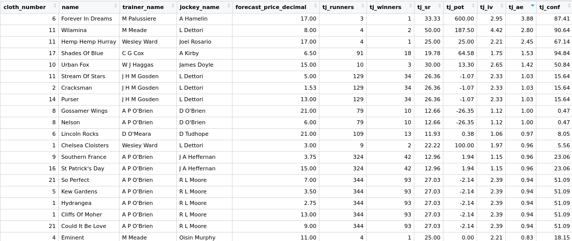
Today we’re going to look at measuring sire strike rates and ranking them, a method which has been doing quite well so far this Royal Ascot. Of the two 2 year old races so far, on Tuesday, the top contender by sire strike rate sire produced the winner of the Coventry Stakes in Calyx at 2/1.
Here’s a screenshot of the query results for the Coventry:
![]()
Yesterday, Wednesday, saw the joint top sire strike rate produce the second in Gossamer Wings at 25/1, and the fourth, So Perfect, at 8/1. Another screenshot of the query follows:
![]()
Sod’s law says that today will be the day that the two year old sires system fails, since that happens all the time in betting – and of course there is no such thing as a sure thing. But there is such a thing as gaining an “an edge” with a method or a combination of methods. The edge needs to be measured and weighed up against the prices on offer to see if there is value, but that’s not what today’s post is about – it’s about a method to generate a possible edge in the first place.
We can also pick holes in ranking anything by strike rate. The winner on day 1 included its own previous win in the very small sample size – because, as a sire, Kingman’s progency have not yet had many runs.
But given those warnings, there is usually little influence of the horse itself in this method, particularly when there is a large sample of previous runs. Also, on the question of sample size, it’s possible to overcome the problem of small samples by applying some simple Bayesian priors to augment the winner and runner ratios – but more about that as well on another day.
So without further ado, here is today’s ranking of horses by sire strike rate for the Norfolk Stakes. Only 10 runners, so not such a cavalry charge as the first two days, and also note very narrow variance between strike rates, with a low strike rate at 11%, as top.
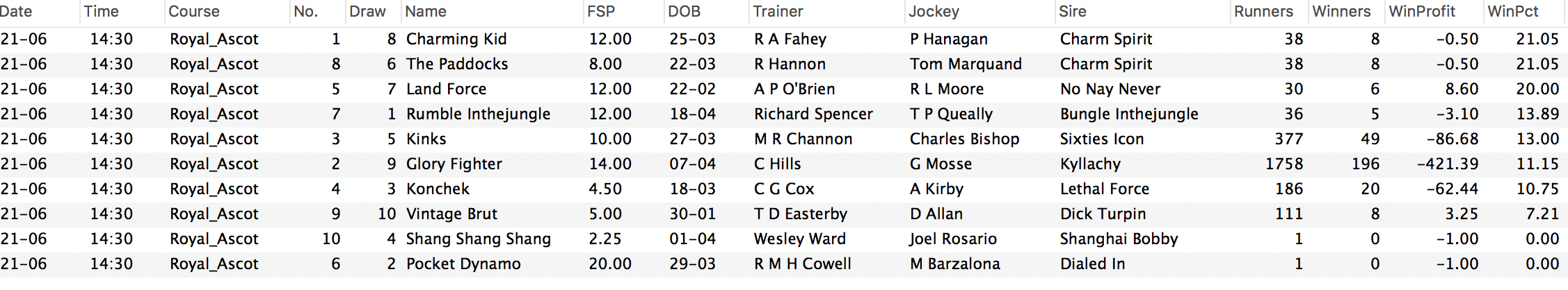
And – since it’s better to teach a man to fish, here is the Smartform query that subscribers can run for themselves for the rest of Royal Ascot.
--  Select the flat turf races for 2yos today at Ascot with selected columns from the daily races and runers tables

--  Note Database lists the course as Royal_Ascot so looking for all races with Ascot in the course hense using like  with %


DROP TABLE IF EXISTS today_2yoturf_races;
CREATE TABLE today_2yoturf_races AS (

select

race_id, meeting_date, scheduled_time, Course, cloth_number, name, foaling_date, sire_name ,
forecast_price_decimal, Trainer_Name Trainer, Jockey_Name Jockey, Stall_Number Draw
from daily_races
join daily_runners using (race_id)
where meeting_date > curdate()

and race_type = 'flat'
and track_type = 'turf'
and age_range  = '2YO only'
and course like  '%Ascot%'     );


--   Create history for 2yo turf sires
--

DROP TABLE IF EXISTS hist_2yoturf_sires;

CREATE TABLE hist_2yoturf_sires AS (

select z.sire_name   ,
COUNT(*) AS Runners,
SUM(winner) AS Winners,
sum(WinProfit)  as WinProfit,

ROUND(((SUM(CASE WHEN z.finish_position = 1 THEN 1 ELSE 0 END) / COUNT(*)) * 100),2) AS WinPct,
case when SUM(winner) = 0 then NULL else
round((SUM(CASE WHEN z.winner = 1 THEN z.distance_yards ELSE 0 END)/220) / SUM( z.winner  ),1) END AS AveWinDist,
sum(Placer) as Placers,
sum(PLaceProfit) as PlaceProfit,

ROUND(((SUM(CASE WHEN z.Placer = 1 THEN 1 ELSE 0 END) / COUNT(*)) * 100),2) AS PlacePct,

case when SUM(placer) = 0 then NULL else

round((SUM(CASE WHEN z.Placer = 1 THEN z.distance_yards ELSE 0 END)/220) / SUM( z.Placer  ),1) END AS AvePlaceDist

from (

select
hru.sire_name , hra.distance_yards,hru.starting_price_decimal,hru.days_since_ran , hra.class, hru.finish_position ,
case when hru.finish_position = 1 then 1 else 0 end as Winner,
case when num_runners < 8 then case when finish_position in ( 2) then 1 else 0 end

else

case when num_runners < 16 then case when finish_position in ( 2,3) then 1 else 0 end

else

case when handicap = 1 then case when finish_position in (2,3,4) then 1 else 0 end

else

case when finish_position in ( 1,2,3) then 1 else 0 end

end end end as Placer,

round(CASE WHEN finish_position = 1 THEN (starting_price_decimal -1) ELSE -1 END,2) AS WinProfit,

round(case when (

Case when num_runners < 5 then case when finish_position = 1 then 1 else 0 end

else

case when num_runners < 8 then case when finish_position in ( 1,2)  then 1 else 0 end

else

case when num_runners < 16 then case when finish_position in ( 1,2,3)  then 1 else 0 end

else

case when handicap = 1 then case when finish_position in (1,2,3,4) then 1 else 0 end

else

case when finish_position in ( 1,2,3)  then 1 else 0

end end end end end )

= 1

then (starting_price_decimal -1) /

Case when num_runners < 5 then 1

else

case when num_runners < 8 then 4

else

case when num_runners < 12 then 5

else

case when handicap = 1 then 4 else 5

end end end end else -1 end,2)

PlaceProfit

from today_2yoturf_races
join  historic_runners hru using (sire_name)
join historic_races hra on hru.race_id = hra.race_id

where hra.race_type_Id = 12
and hra.max_age = 2

and in_race_comment <> 'Withdrawn'
and starting_price_decimal IS NOT NULL

) z


group by z.sire_name
order by z.sire_name);


--

--   Create current 2yo turf runners with sire stats

select CONCAT(substr(tdr.scheduled_time, 9, 2),'-',substr(tdr.scheduled_time, 6, 2)) as Date,

substr(tdr.scheduled_time, 11, 6) as Time, tdr.course as Course,

tdr.cloth_number as 'No.',  Draw, tdr.name as Name,
case when tdr.forecast_price_decimal is NULL then 'Res' else tdr.forecast_price_decimal - 1 end as FSP,

CONCAT(substr(tdr.foaling_date, 9, 2),'-',substr(tdr.foaling_date, 6, 2)) as DOB,

Trainer,  Jockey,
tds.sire_name Sire, tds.Runners,
tds.Winners, tds.WinProfit, tds.WinPct, IFNULL(tds.AveWinDist,'-') AveWinDist,
tds.Placers, tds.PlaceProfit, tds.PlacePct, IFNULL(tds.AvePlaceDist,'-') AvePlaceDist

from today_2yoturf_races tdr

left join hist_2yoturf_sires tds using (sire_name)
order by tdr.scheduled_time,   tdr.course, tds.WinPct desc;
The notes in the query tell you what’s going on at every stage. Copy and paste this query into your favourite MySQL client – Heidi, MySQL Workbench, or Sequel Pro on Mac – and after a few seconds you’ll have the top contenders for tomorrow’s two year old racing, too.
Loops With R – Creating a Racecard with Trainer and Jockey Stats
Tuesday, June 19th, 2018Yesterday we looked at how to create a function in order to easily run the same set of code multiple times, without having to manually edit the code every time. While this is a highly useful concept to understand, we’re still left with manually applying the trainer and jockey combinations for each runner. It remains a time consuming task. Therefore, this article covers creating a basic for loop to iterate over the rows of a dataframe and apply a function to each of them.
There are many ways to loop over the rows of a dataframe, list or matrix in R. Some methods are more efficient than others, while some are perhaps more logical than others. Specifically this article demonstrates how to apply a for loop, which rightly receives some criticism for being slow to execute in certain circumstances. For our purposes, with a limited number of rows, this will not be a problem. However, the reader should investigate R’s apply family of functions and also the map function in the purrr library.
The full R code will be provided within the article, as there have been some useful changes made to code used previously. The complete code will also, as usual, be provided at the end of this article.
Begin by returning historic racing results, this time since 2013 for a full five year dataset and also from tomorrow’s race card:
# Load the library packages
library("RMySQL")
library("dplyr")

# Connect to the Smartform database. Substitute the placeholder credentials for your own.
# The IP address can be substituted for a remote location if appropriate.
con <- dbConnect(MySQL(),
                 host='127.0.0.1',
                 user='yourusername',
                 password='yourpassword',
                 dbname='smartform')

# Select relevant historic results
sql1 <- paste("SELECT historic_races.course,
              historic_races.meeting_date,
              historic_races.conditions,
              historic_races.group_race,
              historic_races.race_type_id,
              historic_races.race_type,
              historic_runners.name,
              historic_runners.jockey_name,
              historic_runners.trainer_name,
              historic_runners.finish_position,
              historic_runners.starting_price_decimal
              FROM smartform.historic_runners
              JOIN smartform.historic_races USING (race_id)
              WHERE historic_races.meeting_date >= '2012-01-01'", sep="")

smartform_results <- dbGetQuery(con, sql1)

# Select relevant daily results for tomorrow
sql2 <- paste("SELECT daily_races.course,
              daily_races.race_title,
              daily_races.meeting_date,
              daily_runners.cloth_number,
              daily_runners.name,
              daily_runners.trainer_name,
              daily_runners.jockey_name,
              daily_runners.forecast_price_decimal
              FROM smartform.daily_races
              JOIN smartform.daily_runners USING (race_id)
              WHERE daily_races.meeting_date >='2018-06-20'", sep="")

smartform_daily_results <- dbGetQuery(con, sql2)

dbDisconnect(con)
Next is the Trainer/Jockey function explained yesterday. However, the code will be broken into a few sections, as there have been some changes incorporated.
The function, as detailed previously:
# Name the function and add some arguments
tj <- function(race_filter = "", price_filter = 1000, trainer, jockey){

  # Filter for flat races only
  flat_races_only <- dplyr::filter(smartform_results,
                                   race_type_id == 12 |
                                     race_type_id == 15)

  # Add an if else statement for the race_filter argument
  if (race_filter == "group"){

    filtered_races <- dplyr::filter(flat_races_only,
                                    group_race == 1 |
                                      group_race == 2 |
                                      group_race == 3 )
  } else {

    filtered_races = flat_races_only
  }

  # Filter by trainer name
  trainer_filtered <- dplyr::filter(filtered_races,
                                    grepl(trainer, trainer_name))

  # Remove non-runners
  trainer_name_filtered <- dplyr::filter(trainer_filtered, !is.na(finish_position))

  # Filter by jockey name
  trainer_jockey_filtered <- dplyr::filter(trainer_filtered,
                                           grepl(jockey, jockey_name))

  # Filter by price
  trainer_jockey_price_filtered <- dplyr::filter(trainer_jockey_filtered,
                                                 starting_price_decimal <= price_filter)

  #  Calculate Profit and Loss
  trainer_jockey_cumulative <- cumsum(
    ifelse(trainer_jockey_price_filtered$finish_position == 1,
           (trainer_jockey_price_filtered$starting_price_decimal-1),
           -1)
  )

  # Calculate Strike Rate
  winners <- nrow(dplyr::filter(trainer_jockey_price_filtered,
                                finish_position == 1))

  runners <- nrow(trainer_jockey_price_filtered)

  strike_rate <- (winners / runners) * 100

  # Calculate Profit on Turnover or Yield
  profit_on_turnover <- (tail(trainer_jockey_cumulative, n=1) / runners) * 100

  # Check if POT is zero length to catch later errors
  if (length(profit_on_turnover) == 0) profit_on_turnover <- 0
The last line above is new. This line is being used to catch any instances where the profit on turnover figure is of zero length. That means that the calculation has not been successful, usually because there were no runners for the combination of trainer and jockey.
Continuing with the function:
  # Calculate Impact Values
  # First filter all runners by price, to return those just starting at the price_filter or less
  all_runners <- nrow(dplyr::filter(filtered_races,
                                    starting_price_decimal <= price_filter))

  # Filter all winners by the price filter
  all_winners <- nrow(dplyr::filter(filtered_races,
                                    finish_position == 1 &
                                      starting_price_decimal <= price_filter))

  # Now calculate the Impact Value
  iv <- (winners / all_winners) / (runners / all_runners)

  # Calculate Actual vs Expected ratio
  # # Convert all decimal odds to probabilities
  total_sp <- sum(1/trainer_jockey_price_filtered$starting_price_decimal)

  # Calculate A/E by dividing the number of  winners, by the sum of all SP probabilities.
  ae <- winners / total_sp

  # Calculate Archie
  archie <- (runners * (winners  - total_sp)^2)/ (total_sp  * (runners - total_sp))

  # Calculate the Confidence figure
  conf <- pchisq(archie, df = 1)*100

  # Create an empty variable
  trainer_jockey <- NULL

  # Add all calculated figures as named objects to the variable, which creates a list
  trainer_jockey$tj_runners <- runners
  trainer_jockey$tj_winners <- winners
  trainer_jockey$tj_sr <- strike_rate
  trainer_jockey$tj_pot <- profit_on_turnover
  trainer_jockey$tj_iv <- iv
  trainer_jockey$tj_ae <- ae
  trainer_jockey$tj_conf <- conf

  # Add an error check to convert all NaN values to zero
  final_results <- unlist(trainer_jockey)
  final_results[ is.nan(final_results) ] <- 0

  # Manipulate the layout of returned results to be a nice dataframe
  final_results <- t(as.data.frame(final_results))
  rownames(final_results) <- c()

  # 2 decimal places only
  round(final_results, 2)

  # Finally, close the function
}
Once again, there are some new lines in the final part of the function above. The results are checked for NaN values, which again occur if a calculation has failed. It is not possible, for example, to calculate strike rate if there are no runners for the trainer and jockey combination. Error checking such as this will take some time to implement, but does save a lot of headaches later.
The results are then transformed, with t from a long to wide dataframe, the rownames are removed and all results rounded to two decimal places.
Now, we move on to the new section for this article. First, filter the current daily races for Group races only and also create an empty placeholder list.
# Filter tomorrow's races for Group races only
group_races_only <- dplyr::filter(smartform_daily_results,
                                  grepl(paste(c("Group 1", "Group 2", "Group 3"), collapse="|"), race_title))

# Create a placeholder list which will be required later
row <- list()
Then start the for loop, which essentially says for every value of name, which is the column containing the horse’s name, apply the code which follows. This code includes extracing the trainer and jockey names, then executing the function defined earlier. Lastly, the data is iteratively added to the emtpy list and converted to a dataframe.
# Setup the loop
# For each horse in the group_races_only dataframe
for (i in group_races_only$name) {

  runner_details = group_races_only[group_races_only$name==i,]

  # Extract trainer and jockey names
  trainer = runner_details$trainer_name
  jockey = runner_details$jockey_name

  # Apply the Trainer/Jockey function for Group races only
  trainer_jockey_combo <- tj(race_filter = "group",
                             trainer = trainer,
                             jockey = jockey)

  # Add results row by row to the previously defined list
  row[[i]] <- trainer_jockey_combo

  # Create a final dataframe
  stats_final <- as.data.frame(do.call("rbind", row))

}
As a final piece of code, we bind the new data and the general racing data from the Smartform database in a new variable called racecard. Viewing this racecard will now display the strike rate, profit on turnover, impact value, actual vs expected and confidence figure for every jockey and trainer combination in Group races on tomorrow’s race card. They are of course all at Royal Ascot.
# Create a new variable called racecard. Bind together the generic race details with the newly created stats
racecard <- cbind(group_races_only,stats_final)
This data can now be reviewed for interesting angles. The screenshot below displays the data ordered descending from the highest A/E value. The first thing to notice about the top three entries is the very small sample size, with only three of four runs. However, the fourth entry for Cox and Kirby does have a robust sample size and some very good figures. Shades of Blue in the Queen Mary Stakes tomorrow at Royal Ascot is certainly worth a closer look. As are the Gosden and Dettori trio of Stream of Stars, Cracksman and Purser. This combination already struck three times today with Calyx, Without Parole and Monarch’s Glen.
Good luck!
Questions and queries about this article should be posted as a comment below or on the Betwise Q&A board.
The full R code used in this article is found below.
# Load the library packages
library("RMySQL")
library("dplyr")

# Connect to the Smartform database. Substitute the placeholder credentials for your own.
# The IP address can be substituted for a remote location if appropriate.
con <- dbConnect(MySQL(),
                 host='127.0.0.1',
                 user='yourusername',
                 password='yourpassword',
                 dbname='smartform')

# Select relevant historic results
sql1 <- paste("SELECT historic_races.course,
              historic_races.meeting_date,
              historic_races.conditions,
              historic_races.group_race,
              historic_races.race_type_id,
              historic_races.race_type,
              historic_runners.name,
              historic_runners.jockey_name,
              historic_runners.trainer_name,
              historic_runners.finish_position,
              historic_runners.starting_price_decimal
              FROM smartform.historic_runners
              JOIN smartform.historic_races USING (race_id)
              WHERE historic_races.meeting_date >= '2012-01-01'", sep="")

smartform_results <- dbGetQuery(con, sql1)

# Select relevant daily results for tomorrow
sql2 <- paste("SELECT daily_races.course,
              daily_races.race_title,
              daily_races.meeting_date,
              daily_runners.cloth_number,
              daily_runners.name,
              daily_runners.trainer_name,
              daily_runners.jockey_name,
              daily_runners.forecast_price_decimal
              FROM smartform.daily_races
              JOIN smartform.daily_runners USING (race_id)
              WHERE daily_races.meeting_date >='2018-06-20'", sep="")

smartform_daily_results <- dbGetQuery(con, sql2)

dbDisconnect(con)

# Name the function and add some arguments
tj <- function(race_filter = "", price_filter = 1000, trainer, jockey){

  # Filter for flat races only
  flat_races_only <- dplyr::filter(smartform_results,
                                   race_type_id == 12 |
                                     race_type_id == 15)

  # Add an if else statement for the race_filter argument
  if (race_filter == "group"){

    filtered_races <- dplyr::filter(flat_races_only,
                                    group_race == 1 |
                                      group_race == 2 |
                                      group_race == 3 )
  } else {

    filtered_races = flat_races_only
  }

  # Filter by trainer name
  trainer_filtered <- dplyr::filter(filtered_races,
                                    grepl(trainer, trainer_name))

  # Remove non-runners
  trainer_name_filtered <- dplyr::filter(trainer_filtered, !is.na(finish_position))

  # Filter by jockey name
  trainer_jockey_filtered <- dplyr::filter(trainer_filtered,
                                           grepl(jockey, jockey_name))

  # Filter by price
  trainer_jockey_price_filtered <- dplyr::filter(trainer_jockey_filtered,
                                                 starting_price_decimal <= price_filter)

  #  Calculate Profit and Loss
  trainer_jockey_cumulative <- cumsum(
    ifelse(trainer_jockey_price_filtered$finish_position == 1,
           (trainer_jockey_price_filtered$starting_price_decimal-1),
           -1)
  )

  # Calculate Strike Rate
  winners <- nrow(dplyr::filter(trainer_jockey_price_filtered,
                                finish_position == 1))

  runners <- nrow(trainer_jockey_price_filtered)

  strike_rate <- (winners / runners) * 100

  # Calculate Profit on Turnover or Yield
  profit_on_turnover <- (tail(trainer_jockey_cumulative, n=1) / runners) * 100

  # Check if POT is zero length to catch later errors
  if (length(profit_on_turnover) == 0) profit_on_turnover <- 0

  # Calculate Impact Values
  # First filter all runners by price, to return those just starting at the price_filter or less
  all_runners <- nrow(dplyr::filter(filtered_races,
                                    starting_price_decimal <= price_filter))

  # Filter all winners by the price filter
  all_winners <- nrow(dplyr::filter(filtered_races,
                                    finish_position == 1 &
                                      starting_price_decimal <= price_filter))

  # Now calculate the Impact Value
  iv <- (winners / all_winners) / (runners / all_runners)

  # Calculate Actual vs Expected ratio
  # # Convert all decimal odds to probabilities
  total_sp <- sum(1/trainer_jockey_price_filtered$starting_price_decimal)

  # Calculate A/E by dividing the number of  winners, by the sum of all SP probabilities.
  ae <- winners / total_sp

  # Calculate Archie
  archie <- (runners * (winners  - total_sp)^2)/ (total_sp  * (runners - total_sp))

  # Calculate the Confidence figure
  conf <- pchisq(archie, df = 1)*100

  # Create an empty variable
  trainer_jockey <- NULL

  # Add all calculated figures as named objects to the variable, which creates a list
  trainer_jockey$tj_runners <- runners
  trainer_jockey$tj_winners <- winners
  trainer_jockey$tj_sr <- strike_rate
  trainer_jockey$tj_pot <- profit_on_turnover
  trainer_jockey$tj_iv <- iv
  trainer_jockey$tj_ae <- ae
  trainer_jockey$tj_conf <- conf

  # Add an error check to convert all NaN values to zero
  final_results <- unlist(trainer_jockey)
  final_results[ is.nan(final_results) ] <- 0

  # Manipulate the layout of returned results to be a nice dataframe
  final_results <- t(as.data.frame(final_results))
  rownames(final_results) <- c()

  # 2 decimal places only
  round(final_results, 2)

  # Finally, close the function
}

# Filter tomorrow's races for Group races only
group_races_only <- dplyr::filter(smartform_daily_results,
                                  grepl(paste(c("Group 1", "Group 2", "Group 3"), collapse="|"), race_title))

# Create a placeholder list which will be required later
row <- list()

# Setup the loop
# For each horse in the group_races_only dataframe
for (i in group_races_only$name) {


  runner_details = group_races_only[group_races_only$name==i,]

  # Extract trainer and jockey names
  trainer = runner_details$trainer_name
  jockey = runner_details$jockey_name

  # Apply the Trainer/Jockey function for Group races only
  trainer_jockey_combo <- tj(race_filter = "group",
                             trainer = trainer,
                             jockey = jockey)

  # Add results row by row to the previously defined list
  row[[i]] <- trainer_jockey_combo

  # Create a final dataframe
  stats_final <- as.data.frame(do.call("rbind", row))

}

# Create a new variable called racecard. Bind together the generic race details with the newly created stats
racecard <- cbind(group_races_only,stats_final)
Creating Functions with R – using trainer and jockey combinations
Monday, June 18th, 2018In the previous article we looked at how to calculate some useful figures such as profit on turnover, impact values, actual vs expected, Archie and a confidence figure regarding how much luck was involved in the returned figures. The code demonstrated works well, but can be cumbersome to easily alter items such as trainer, jockey or price filters.
Fortunately the R language supports creation of user defined functions. A function is essentially a wrapper around a set of code routines, which are executed when the function is called at a later time. This makes it very easy to re-run the same code multiple times, using specific arguments to alter the results. Sounds difficult? It’s not really. Much of the R code we’re already familiar with, such as dplyr::filter are functions themselves. If you ever find yourself writing the same R code snippet more than three times in a larger program or script, think about how to create a function instead.
The goal of the function described in this article is to return a set of results for a specific trainer and jockey combination, with some additional argument options added.
The code examples again assume data has already been returned from the Smartform database and is contained in a variable called smartform_results. Also assumed is that part of the initial MySQL query was to limit results to those only since January, 1st, 2016. Full R code will be provided at the end of this article.
The first step is to define the function name and arguments.
# Name the function and add some arguments
tj <- function(race_filter = "", price_filter = 1000, trainer, jockey){
The function is now named tj for Trainer and Jockey. The function has four defined arguments. A race filter, a price filter and arguments for trainer and jockey. If a value is not defined for a function argument, the user must include and define the argument when calling the function. This is the case for trainer and jockey above. However, default values for arguments may be specified. In the above code the race_filter has an empty default value, for all races, and the price_filter is defined as 1000, which is the maximum possible price on Betfair, thus also including all possible prices when applied as a less than or equal to fitler.
Now, we begin the remainder of our function, which is essentially the same code as previously, with some additional changes to account for the function arguments.
# Filter for flat races only
flat_races_only <- dplyr::filter(smartform_results,
                                 race_type_id == 12 |
                                   race_type_id == 15)

# Add an if/else statement for the race_filter argument
if (race_filter == "group"){

filtered_races <- dplyr::filter(flat_races_only,
                                  group_race == 1 |
                                    group_race == 2 |
                                    group_race == 3 )
} else {

  filtered_races = flat_races_only
}
The if else statement above is another new concept. It states that if the race_filter equals the word group apply one set of code, otherwise (else) run a different set of code. In the case of the current function, only one race_filter is supported, that is filter by Group races only or return results from all races. Additional race filters, such as class or age perhaps, could also be added to the function through additional else options.
The next block of code should be largely familiar from the previous article.
# Filter by trainer name
trainer_filtered <- dplyr::filter(filtered_races,
                                         grepl(trainer, trainer_name))

# Remove non-runners
trainer_name_filtered <- dplyr::filter(trainer_filtered, !is.na(finish_position))

# Filter by jockey name
trainer_jockey_filtered <- dplyr::filter(trainer_filtered,
                                               grepl(jockey, jockey_name))

# Filter by price
trainer_jockey_price_filtered <- dplyr::filter(trainer_jockey_filtered,
                                               starting_price_decimal <= price_filter)
The above lines now filter by the values provided in the arguments trainer, jockey and price_filter. If values for trainer and jockey are not provided by the user, and because no defaults were supplied, the function will fail. Also, if an incorrect name, which does not match values in the dataset, is supplied the function will also fail. There is no error checking provided in this example code. The price_filter was provided with a default value of 1000 and therefore if the user does not define it, the function will return all values equal to or less than 1000.
The next blocks of code are once again very similar to that used previously when calculating the statistics we’re interested in.
#  Calculate Profit and Loss
trainer_jockey_cumulative <- cumsum(
  ifelse(trainer_jockey_price_filtered$finish_position == 1,
         (trainer_jockey_price_filtered$starting_price_decimal-1),
         -1)
)

# Calculate Strike Rate
winners <- nrow(dplyr::filter(trainer_jockey_price_filtered,
                                           finish_position == 1))

runners <- nrow(trainer_jockey_price_filtered)


strike_rate <- (winners / runners) * 100

# Calculate Profit on Turnover or Yield
profit_on_turnover <- (tail(trainer_jockey_cumulative, n=1) / runners) * 100


# Calculate Impact Values
# First filter all runners by price, to return those just starting at the price_filter or less
all_runners <- nrow(dplyr::filter(filtered_races,
                                        starting_price_decimal <= price_filter))

# Filter all winners by the price filter
all_winners <- nrow(dplyr::filter(filtered_races,
                                        finish_position == 1 &
                                          starting_price_decimal <= price_filter))

# Now calculate the Impact Value
iv <- (winners / all_winners) / (runners / all_runners)

# Calculate Actual vs Expected ratio
# # Convert all decimal odds to probabilities
total_sp <- sum(1/trainer_jockey_price_filtered$starting_price_decimal)

# Calculate A/E by dividing the number of  winners, by the sum of all SP probabilities.
ae <- winners / total_sp

# Calculate Archie
archie <- (runners * (winners  - total_sp)^2)/ (total_sp  * (runners - total_sp))

# Calculate the Confidence figure
conf <- pchisq(archie, df = 1)*100
That covers all the calculations. Now we return the results in a nice dataframe.
# Create an empty variable
trainer_jockey <- NULL

# Add all calculated figures as named objects to the variable, which creates a list
trainer_jockey$runners <- runners
trainer_jockey$winners <- winners
trainer_jockey$sr <- strike_rate
trainer_jockey$pot <- profit_on_turnover
trainer_jockey$iv <- iv
trainer_jockey$ae <- ae
trainer_jockey$conf <- conf

# Convert and return as a dataframe
as.data.frame(trainer_jockey)

# Finally, close the function
}
The last line here is very important and should not be forgotten. The curly bracket was used to start the function at the beginning, and therefore the matching closing curly bracket must be used at the end.
We now have a trainer/jockey function defined. How do we use it? Simply call the function, with defined arguments. Using the previous filters of Aiden O’Brien trained runners, ridden by Ryan Moore, in Group races and starting at a price of 4.0 or less, we do the following:
# Run the function with arguments and store in a results object
results <- tj(race_filter = "group",
              price_filter = 4.0,
              trainer = "A P O'Brien",
              jockey = "R L Moore")

# Show results
results

  runners winners       sr      pot       iv       ae    conf
1     137      66 48.17518 13.62774 1.279968 1.069609 53.9223
This matches the results previously obtained when running through the code manually. Tomorrow in the Group 1 Queen Anne Stakes at Royal Ascot, Rhododendron is trained by Aiden O’Brien, ridden by Ryan Moore and is currently 3/1, thus matching the filters used in this function.
Now the function is defined, it is easy to start looking at alternative filter sets, without having to manually adjust any code. Some examples are outlined below:
# No price filter, which works because a default of 1000 was defined in the function
results_no_price <- tj(race_filter = "group",
                       trainer = "A P O'Brien",
                       jockey = "R L Moore")

  runners winners       sr      pot       iv       ae     conf
1     246      78 31.70732 -3.04878 2.825292 1.004775 4.056167

# All races, not just Group, with a price filter of 4.0
results_all_races <- tj(price_filter = 4.0,
                        trainer = "A P O'Brien",
                        jockey = "R L Moore")

  runners winners       sr      pot       iv        ae     conf
1     227     100 44.05286 2.718062 1.343485 0.9936154 6.841419

# All races and no price filter for this trainer and jockey combination
results_all_races_no_price <- tj(trainer = "A P O'Brien",
                                 jockey = "R L Moore")

  runners winners       sr       pot       iv        ae     conf
1     387     119 30.74935 -8.183463 2.919438 0.9519335 48.63522
Also keep in mind these results are only since January 1st, 2016 as this filter was previously defined in the original SQL query. Hopefully, it should be reasonably clear how to add a date argument to extend this function.
Finally, if we wanted to investigate alternative trainer and jockey combinations, this is also quite easy now the function is already defined.
# David Simcock and Oisin Murphy together in Group races
simcock_murphy <- tj(race_filter = "group",
                    trainer = "D M Simcock",
                    jockey = "Oisin Murphy")

  runners winners      sr       pot        iv        ae     conf
1      21       2 9.52381 -66.66667 0.8486226 0.9350056 7.989577
David Simcock and Oisin Murphy team up with Lightning Spear, also in the Queen Anne at Ascot.
Good luck at the big meeting tomorrow!
Questions and queries about this article should be posted as a comment below or on the Betwise Q&A board.
The full R code used in this article is found below.
# Load the RMySQL library package
library("RMySQL")
library("dplyr")

# Connect to the Smartform database. Substitute the placeholder credentials for your own.
# The IP address can be substituted for a remote location if appropriate.
con <- dbConnect(MySQL(),
                        host='127.0.0.1',
                        user='yourusername',
                        password='yourpassword',
                        dbname='smartform')

sql1 <- paste("SELECT historic_races.course,
              historic_races.meeting_date,
              historic_races.conditions,
              historic_races.group_race,
              historic_races.race_type_id,
              historic_races.race_type,
              historic_runners.name,
              historic_runners.jockey_name,
              historic_runners.trainer_name,
              historic_runners.finish_position,
              historic_runners.starting_price_decimal
              FROM smartform.historic_runners
              JOIN smartform.historic_races USING (race_id)
              WHERE historic_races.meeting_date >= '2016-01-01'", sep="")

smartform_results <- dbGetQuery(con, sql1)

dbDisconnect(con)

# Name the function and add some arguments
tj <- function(race_filter = "", price_filter = 1000, trainer, jockey){

# Filter for flat races only
flat_races_only <- dplyr::filter(smartform_results,
                                 race_type_id == 12 |
                                   race_type_id == 15)

# Add an if else statement for the race_filter argument
if (race_filter == "group"){

filtered_races <- dplyr::filter(flat_races_only,
                                  group_race == 1 |
                                    group_race == 2 |
                                    group_race == 3 )
} else {

  filtered_races = flat_races_only
}

# Filter by trainer name
trainer_filtered <- dplyr::filter(filtered_races,
                                         grepl(trainer, trainer_name))

# Remove non-runners
trainer_name_filtered <- dplyr::filter(trainer_filtered, !is.na(finish_position))

# Filter by jockey name
trainer_jockey_filtered <- dplyr::filter(trainer_filtered,
                                               grepl(jockey, jockey_name))

# Filter by price
trainer_jockey_price_filtered <- dplyr::filter(trainer_jockey_filtered,
                                               starting_price_decimal <= price_filter)

#  Calculate Profit and Loss
trainer_jockey_cumulative <- cumsum(
  ifelse(trainer_jockey_price_filtered$finish_position == 1,
         (trainer_jockey_price_filtered$starting_price_decimal-1),
         -1)
)

# Calculate Strike Rate
winners <- nrow(dplyr::filter(trainer_jockey_price_filtered,
                                           finish_position == 1))

runners <- nrow(trainer_jockey_price_filtered)

strike_rate <- (winners / runners) * 100

# Calculate Profit on Turnover or Yield
profit_on_turnover <- (tail(trainer_jockey_cumulative, n=1) / runners) * 100

# Calculate Impact Values
# First filter all runners by price, to return those just starting at the price_filter or less
all_runners <- nrow(dplyr::filter(filtered_races,
                                        starting_price_decimal <= price_filter))

# Filter all winners by the price filter
all_winners <- nrow(dplyr::filter(filtered_races,
                                        finish_position == 1 &
                                          starting_price_decimal <= price_filter))

# Now calculate the Impact Value
iv <- (winners / all_winners) / (runners / all_runners)

# Calculate Actual vs Expected ratio
# # Convert all decimal odds to probabilities
total_sp <- sum(1/trainer_jockey_price_filtered$starting_price_decimal)

# Calculate A/E by dividing the number of  winners, by the sum of all SP probabilities.
ae <- winners / total_sp

# Calculate Archie
archie <- (runners * (winners  - total_sp)^2)/ (total_sp  * (runners - total_sp))

# Calculate the Confidence figure
conf <- pchisq(archie, df = 1)*100

# Create an empty variable
trainer_jockey <- NULL

# Add all calculated figures as named objects to the variable, which creates a list
trainer_jockey$runners <- runners
trainer_jockey$winners <- winners
trainer_jockey$sr <- strike_rate
trainer_jockey$pot <- profit_on_turnover
trainer_jockey$iv <- iv
trainer_jockey$ae <- ae
trainer_jockey$conf <- conf

# Convert and return as a dataframe
as.data.frame(trainer_jockey)

# Finally, close the function
}
Further Calculations using R to analyse the performance of jockeys and trainers
Friday, June 1st, 2018Last week we explored some visual ways in which to analyse performance. This included representations such as line charts, scatterplots and regression fits. This week we examine some mathematical and statistical approaches to expand on the simple calculations of strike rate and profit & loss.
A positive profit & loss is obviously critical in making money from a series of bets. A negative profit & loss largely renders everything else irrelevant. However, a simple positive profit & loss calculation still does not expose the full story. Imagine a positive profit of 20 points, from a series of 1000 bets. Is that a good or bad performance? A calculation of Profit on Turnover (POT) or Yield can assist.
Again, we’ll use the combination of Aiden O’Brien and Ryan Moore, in Group Races only, since the beginning of 2016, with a filter of less than or equal to 4.00 starting price, as the example dataset. The code examples again assume data has already been returned from the Smartform database and is contained in a variable called smartform_results. Also assumed is that part of the initial MySQL query was to limit results to those only since January, 1st, 2016. Full R code will be provided at the end of this article.
# Filter for flat races only
flat_races_only <- dplyr::filter(smartform_results,
                                 race_type_id == 12 |
                                   race_type_id == 15)
# Filter for Group races only
group_races_only <- dplyr::filter(flat_races_only,
                                  group_race == 1 |
                                    group_race == 2 |
                                    group_race == 3 )

# Filter for Aiden O'Brien runners only
obrien_group_races_only <- dplyr::filter(group_races_only,
                                         grepl("A P O'Brien", trainer_name))

# Remove non-runners
obrien_group_races_only <- dplyr::filter(obrien_group_races_only, !is.na(finish_position))

# Filter for Ryan Moore rides only
obrien_moore_group_races_only <- dplyr::filter(obrien_group_races_only,
                                               grepl("R L Moore", jockey_name))

# Filter for Starting Prices of 4.00 or less
obrien_moore_group_races_only_price_filter <- dplyr::filter(obrien_moore_group_races_only,
                                                            starting_price_decimal <= 4.0)

# # Calculate Profit and Loss
obrien_moore_cumulative <- cumsum(
  ifelse(obrien_moore_group_races_only_price_filter$finish_position == 1, (obrien_moore_group_races_only_price_filter$starting_price_decimal-1),-1)
)

obrien_moore_group_races_only_price_filter$cumulative <- obrien_moore_cumulative

# Calculate Strike Rate
obrien_moore_winners <- nrow(dplyr::filter(obrien_moore_group_races_only_price_filter,
                                   finish_position == 1))

obrien_moore_runners <- nrow(obrien_moore_group_races_only_price_filter)


strike_rate <- (obrien_moore_winners / obrien_moore_runners) * 100
Detailed explanations of the above calculations have been provided in previous articles. The P&L for the combination examined now stands at 19.67 points, with a Strike Rate of 48.52%.
How good is this in the context of the total amount wagered? Next, calculate Profit on Turnover (POT) or Yield. This is simply the total cumulative profit, divided by the total number of runners and multiplied by 100 to return a percentage.
# Calculate POT
profit_on_turnover <- (tail(obrien_moore_cumulative, n=1) / obrien_moore_runners) * 100
This returns a POT of 14.46%, which is a pretty reasonable figure. A return of almost 15% on an investment would certainly keep many people very happy.
Moving on, there are some other calculations which can assist with providing additional clarity to the overall picture.
The first of these is Impact Value (IV). This measure helps to assertain whether a specific combination of factors returns winners at a higher rate than the rate of winners which did not meet the specific criteria being examined. In our case, we are looking at the performance of Aiden O’Brien trained and Ryan Moore ridden Group runners, with a price filter, versus those Group runners, with the same price filter, who were not trained by Aiden O’Brien and ridden by Ryan Moore. It is worth keeping in mind that IVs are only an indication of the rate of winners, and does not take price into account.
In order to calculate Impact Values, the ratio of the filtered winners to all runners is divided by the ratio of filtered runners to all runners. In our specific case, this is the ratio of O’Brien and Moore winners to all Group winners, starting at a price equal to or less than 4.00, divided by the ratio of O’Brien and Moore runners to all Group Runners, with the same price filter applied.
An Impact Value of greater than 1.0 indicates that the filtered angle in question is outperforming runners in the entire dataset who did meet our filtering criteria.
# Calculate Impact Values
# First filter all Group runners by price, to return those just starting at 4.00 or less
all_group_runners <- nrow(dplyr::filter(group_races_only,
                                        starting_price_decimal <= 4.0))

# Filter all Group winners by the 4.00 price limit
all_group_winners <- nrow(dplyr::filter(group_races_only,
                                        finish_position == 1 &
                                          starting_price_decimal <= 4.0))

# Now calculate the Impact Value
iv <- (obrien_moore_winners / all_group_winners) / (obrien_moore_runners / all_group_runners)
An IV of 1.29 is returned. This is a very healthy result and indicates that the O’Brien and Moore combination generally returns a higher ratio of winners than that of all Group runners, also filtered by the 4.00 or less price.
Finding winners is one thing, making a profit may be something entirely different. Therefore, there is a futher calculation to examine. Now we’ll look at the ratio of Actual vs Expected (A/E) winners, based on probabilties calculated from starting price. This figure will help to inform whether the filtered combination is outperforming market expectations, based on Starting Price probabilities.
A/E is calculated by dividing the number of winners from the filtered dataset, by the sum of all win probabilities. Decimal starting prices first need to be converted to probabilities. Individual starting prices may be converted to probabilities by expressing as a decimal, a fraction with 1 as the numerator and the decimal starting price as the denominator. i.e. 1/Decimal SP or 1/4.0 = 0.25.
# Calculated Actual vs Expected ratio
# Convert all decimal odds to probabilities
total_sp <- sum(1/obrien_moore_group_races_only_price_filter$starting_price_decimal)

# Calculate A/E by dividing the number of all O'Brien and Moore winners, but the sum of all SP probabilities.
obrien_moore_ae <- obrien_moore_winners / total_sp
An A/E figure of 1.07 is returned. Once again, any figure above 1.00 should be viewed positively. If the return is greater than 1.00 it essentially means the filtered dataset is outperforming the market’s expectations. Or, to put it another way, a figure above 1.00 means that the filtered selections win more often than their probabilities (odds) indicate they should. Using a combination like Aiden O’Brien and Ryan Moore it may be somewhat surprising that they perform in excess of market expectations, especially given the regression line seen in last week’s scatterchart, but the A/E figure shows this to be true.
Finally, the last computation included in today’s article is known as Archie. If you are statistically minded, Archie is a variation on the Chi Squared goodness of fit calculation. However, in layman’s terms, Archie provides a figure showing how much the results obtained from a set of data can be attributed to luck. The higher the Archie figure, the less likely the results are down to pure luck. The larger the Archie figure, the better. As a rough guide, an Archie figure of 1.00 still means there is a 32% likelihood the results obtained were due to chance.
I also like to convert the Archie result to a percentage Confidence figure. In this case also, the higher the Confidence figure, the less likely the results are only down to luck.
# Calculate Archie
archie <- (obrien_moore_runners * (obrien_moore_winners  - total_sp)^2)/ (total_sp  * (obrien_moore_runners - total_sp))

# Calculate the Confidence figure
conf <- pchisq(archie, df = 1)*100
In the case of Group race runners, starting at a price of 4.00 or less, trained by Aiden O’Brien and ridden by Ryan Moore, the Confidence figure is almost 60%. This is reasonable, but not particularly strong.
It is worth keeping in mind that Archie and Confidence figures can be seen to change rapidly if the sample data size is only small. Our filtered dataset in this case contains only 136 runners, which is not particularly large.
Further details concerning all these calculations – POT/Yield, IV, A/E and Archie/Confidence – can always be found through Internet searches using popular search engines.
Questions and queries about this article should be posted as a comment below or on the Betwise Q&A board.
The full R code used in this article is found below.
# Load the RMySQL library package
library("RMySQL")
library("dplyr")

# Connect to the Smartform database. Substitute the placeholder credentials for your own.
# The IP address can be substituted for a remote location if appropriate.
con <- dbConnect(MySQL(),
                        host='127.0.0.1',
                        user='yourusername',
                        password='yourpassword',
                        dbname='smartform')

sql1 <- paste("SELECT historic_races.course,
              historic_races.meeting_date,
              historic_races.conditions,
              historic_races.group_race,
              historic_races.race_type_id,
              historic_races.race_type,
              historic_runners.name,
              historic_runners.jockey_name,
              historic_runners.trainer_name,
              historic_runners.finish_position,
              historic_runners.starting_price_decimal
              FROM smartform.historic_runners
              JOIN smartform.historic_races USING (race_id)
              WHERE historic_races.meeting_date >= '2016-01-01'", sep="")

smartform_results <- dbGetQuery(con, sql1)

dbDisconnect(con)

# Filter for flat races only
flat_races_only <- dplyr::filter(smartform_results,
                                 race_type_id == 12 |
                                   race_type_id == 15)
# Filter for Group races only
group_races_only <- dplyr::filter(flat_races_only,
                                  group_race == 1 |
                                    group_race == 2 |
                                    group_race == 3 )

# Filter for Aiden O'Brien runners only
obrien_group_races_only <- dplyr::filter(group_races_only,
                                         grepl("A P O'Brien", trainer_name))

# Remove non-runners
obrien_group_races_only <- dplyr::filter(obrien_group_races_only, !is.na(finish_position))

# Filter for Ryan Moore rides only
obrien_moore_group_races_only <- dplyr::filter(obrien_group_races_only,
                                               grepl("R L Moore", jockey_name))

# Filter for Starting Prices of 4.00 or less
obrien_moore_group_races_only_price_filter <- dplyr::filter(obrien_moore_group_races_only,
                                                            starting_price_decimal <= 4.0)

# # Calculate Profit and Loss
obrien_moore_cumulative <- cumsum(
  ifelse(obrien_moore_group_races_only_price_filter$finish_position == 1, (obrien_moore_group_races_only_price_filter$starting_price_decimal-1),-1)
)

obrien_moore_group_races_only_price_filter$cumulative <- obrien_moore_cumulative

# Calculate Strike Rate
obrien_moore_winners <- nrow(dplyr::filter(obrien_moore_group_races_only_price_filter,
                                   finish_position == 1))

obrien_moore_runners <- nrow(obrien_moore_group_races_only_price_filter)


strike_rate <- (obrien_moore_winners / obrien_moore_runners) * 100

# Calculate POT
profit_on_turnover <- (tail(obrien_moore_cumulative, n=1) / obrien_moore_runners) * 100

# Calculate Impact Values
# First filter all Group runners by price, to return those just starting at 4.00 or less
all_group_runners <- nrow(dplyr::filter(group_races_only,
                                        starting_price_decimal <= 4.0))

# Filter all Group winners by the 4.00 price limit
all_group_winners <- nrow(dplyr::filter(group_races_only,
                                        finish_position == 1 &
                                          starting_price_decimal <= 4.0))

# Now calculate the Impact Value
iv <- (obrien_moore_winners / all_group_winners) / (obrien_moore_runners / all_group_runners)

# Calculated Actual vs Expected ratio
# Convert all decimal odds to probabilities
total_sp <- sum(1/obrien_moore_group_races_only_price_filter$starting_price_decimal)

# Calculate A/E by dividing all O'Brien and Moore winners, but the sum of all SP probabilities.
obrien_moore_ae <- obrien_moore_winners / total_sp

# Calculate Archie
archie <- (obrien_moore_runners * (obrien_moore_winners  - total_sp)^2)/ (total_sp  * (obrien_moore_runners - total_sp))

# Calculate the Confidence figure
conf <- pchisq(archie, df = 1)*100