
New: daily_dams_insights Table Now in Smartform
By colin on Thursday, June 4th, 2026The maternal-line counterpart to our sires table is now available to download — and it lands on the eve of the Epsom Derby meeting, which is no accident.
Following on from last year’s release of daily_sires_insights, we’re pleased to add its natural counterpart to Smartform: daily_dams_insights — the same engineered statistics, viewed down the female line.
The schema is an exact mirror of the sires table. Anything you’ve already built against daily_sires_insights will run against dams with simple field-name substitutions (sire_id → dam_id, sire_name → dam_name, and so on). One row per declared runner, per race, per day; the dam’s other progeny’s prior performance summarised across nine stat groups and four metrics, every aggregate computed strictly from races run before the row’s meeting_date — so it’s feature-correct for any modelling you put it to, with no leakage from the future.
How it sits alongside the sires table
Sire statistics are widely used, and rightly so: coverage is near-total, the samples are large, and a version of them sits in just about every racecard and form product, though the advantage with Smartform remains being able to manipulate them programmatically. The flip side of that ubiquity is that much of what the sire figures tell you is more likely to be reflected in the market already.
The dam line is the opposite proposition. It is half of every runner’s genetic makeup, yet it is rarely queried systematically, and — as the figures below show — it is sparser and noisier than the sire equivalent. That reads like a list of drawbacks; however, it is also the profile of a signal that may still have something left to give: overlooked, under-covered, and seldom mentioned in the form commentary.
What to expect from coverage
We’d rather you see the limits up front than discover them later, so we ran a full coverage audit. Two pictures tell most of the story.
A stallion can cover well over a hundred mares a season; a mare produces roughly one foal a year. That biology shows up directly in the data — there are 20× more distinct dams (71,684) than sires (3,566), but each dam has far fewer offspring to summarise over.
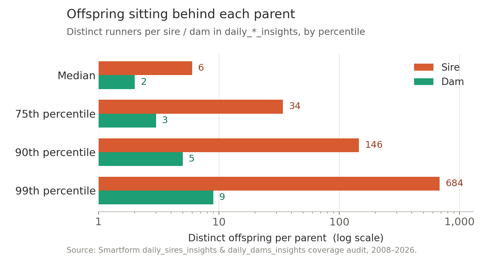
The median sire has 6 offspring in our data; the median dam has 2. The busiest sires reach several hundred; the busiest dams, single figures.
That asymmetry carries through to the sample size behind any individual stat you query. For sires, around 90% of rows rest on 51 or more prior progeny runs at the race type. For dams, that figure is 5%, and most rows sit on a handful of runs.
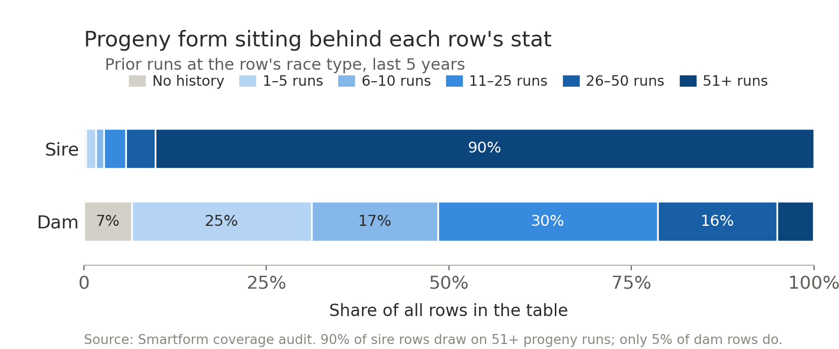
For dams, about 6.5% of rows have no prior history at the exact race type, and roughly a third have five or fewer prior runs to aggregate over.
The practical reading: dam stats are most informative when the dam has multi-offspring history and you stay at the broader race-code level (Flat vs Jumps), where 96.7% of rows have some history and the median row aggregates over 11–25 prior runs. The very specific stats — race-type and course and distance — are sparse enough that you should weight them lightly. A handy guardrail is already in the data: roughly 13% of rows describe a dam whose only progeny in our records is the runner itself, so the dam stat there simply re-states the horse’s own form and adds nothing new. Filter those out with the runs fields and you’re left with genuine sibling signal.
For the record: coverage runs from 2008 across all five UK & Irish race types (Chase, Hurdle, Flat, National Hunt Flat and All-Weather Flat), totalling 2,421,827 rows over 71,684 distinct dams, with dam_id resolved on 99.95% of runners.
Why today, of all days
This isn’t a coincidental release date. Tomorrow brings the Oaks and then on Saturday the Derby – two Classics run over the same 1m4f at Epsom, and two of the best possible test cases for what a maternal-line signal can and can’t do at the very top of the sport.
Our next post – out before racing starts – puts the table straight to work: what the dam data says about past Derby and Oaks trends, and why the two Classics turn out to reward very different reads of a pedigree. It’s a good illustration of using the table in anger.
Get started
Smartform subscribers can download daily_dams_insights now from the downloads section of the site once logged in. (Not yet a subscriber? You’ll need a Smartform subscription first.) Once you’ve installed it, smartform-updater keeps the table current automatically through the standard loaded_at mechanism — exactly as it does your existing tables, with no change to your workflow.
A couple of queries to get going:
-- Today's runners, ranked by their dam's 5-year prior race-type strike rate
SELECT race_id, runner_id, dam_name, rt_5Y_strike_rate, rt_5Y_runs
FROM   daily_dams_insights
WHERE  meeting_date = CURDATE()
ORDER  BY rt_5Y_strike_rate DESC;

-- Dams whose other foals have run today's distance well, with enough runs to trust
SELECT runner_id, dam_name, rt_5Y_distance_prb, rt_5Y_distance_runs
FROM   daily_dams_insights
WHERE  meeting_date = CURDATE()
  AND  rt_5Y_distance_prb  > 65
  AND  rt_5Y_distance_runs >= 5
ORDER  BY rt_5Y_distance_prb DESC;
Full schema and field-level descriptions are linked from the daily_dams_insights page and your Smartform admin area.
As always, questions or suggestions to the usual address. The dam-side breeding signal hasn’t been systematically queryable before now, and we expect you’ll turn up patterns we haven’t looked at yet.
Enjoy!
— Betwise / Smartform
New: Daily Sire Insights – How Today’s Runner Fits the Sire’s Patterns
By colin on Saturday, May 2nd, 2026Introduction
Following on from the recent introduction of Daily Trainer Stats, we’ve extended the same approach to another key area of racing analysis: sire statistics and top performing patterns within the history of each sire’s progeny. Both views are now integrated within a single race view, Daily Trainer & Sire Insights from the top menu on the Betwise website.
The objective is the same – to show Smartform sire data within the context of today’s runners on a race-by-race basis.
For users of Smartform, the full history of sire performance is already available, with data going back to 2008 and covering a wide range of conditions. That level of detail supports deep analysis, model building and backtesting, as well as daily statistics and systems.
Daily Sire Stats complements that by providing a visual, sortable view of how those patterns apply to today’s races, but with a new feature that allows one aspect of sire behaviour to be surfaced clearly – how a sire’s progeny have performed across the spectrum of going.
Built on Smartform: the daily_sires_insights table
As with Daily Trainer Stats, this feature is built on the underlying Smartform data.
In this case, it draws from the daily_sires_insights table, which contains engineered statistics for every runner since March 2008. This dataset summarises how each sire’s progeny have performed across a wide range of conditions, including:
- course and distance
- race type and code
- age group and handicap status
- and multiple timeframes (5-year, 42-day, 21-day)
All figures are calculated on a “to date” basis, meaning they reflect only what would have been known at the time of each race. This makes the data suitable for both live use and historical testing.
On its own, this provides a comprehensive statistical view of sire performance.
But, as with trainer data, a table of figures only tells part of the story in terms of identifying patterns within a sire’s own performance history.
The importance of going
Going is one of the more fundamental influences in racing but one of the most difficult to nail in terms of quantifying its effect. There are several reasons for this, largely to do with how going is measured and reported (more on that shortly). But from a racing record perspective alone, an individual runner rarely shows enough evidence to demonstrate how well or otherwise it handles a certain type of going. If a horse has never raced on extreme going, how do we know if it will handle it? If one race has been run on heavy going and the horse puts in a poor performance, is that enough evidence to say that it doesn’t handle heavy conditions?
On the other hand, it is well understood that horses inherit physical traits from their sire — including aspects of conformation and galloping action — which in turn can influence how they perform under different ground conditions.
This means that going preferences are often reflected consistently across a sire’s progeny, which gives us a much larger data sample from which to infer going preferences:
- For lightly raced horses, where the runner itself may not yet have established any clear profile, this can provide an essential layer of insight.
- And for more exposed runners, it can highlight how they may perform under conditions they have not previously encountered.
Handling the Uncertainty of Going
One of the main challenges in presenting sire data is how to handle going conditions in a meaningful way. We can create a statistic similar to age or recent form that classifies the particular strike rate (or percentage of rivals beaten) for a particular going type that corresponds to past results, however there are limitations to using a single figure since:
- going can change on the day
- pre-race descriptions are not always reliable
- And most importantly a single summary figure that is fixed to one type of going (e.g. Good to Soft) does not provide insight into the sire performance pattern across the range of going, especially adjacent categories such as Good or Soft
A different approach: visualising the full picture
Instead of relying on a single number, Daily Sire Stats uses a similar framework to trainer patterns:
👉 a full distribution of historical performance
But in this case, grouped by:
• going
• and distance bands
Each box plot shows how a sire’s progeny have performed under those conditions, using % rivals beaten (PRB).
And then, for today’s race:
👉 the current runner is placed directly into that distribution (highlighted in red)
This is the key step.
Instead of asking:
“Is this sire good on soft ground?”
You are looking at:
👉 how the sire performs across different goings — and where today’s runner sits within that range
What the Feature Shows – a worked example
For every race, you are presented with:
• A sortable table of sire statistics
• And a set of box plots underneath, specific to each sire
Here we’re looking at the 14.20 from the start of the Guineas meeting (yesterday as we write this post). The table provides a structured overview that can be sorted by a range of different statistics. Here sorted by Mean PRB for the age, going and distance bands (the first metric).
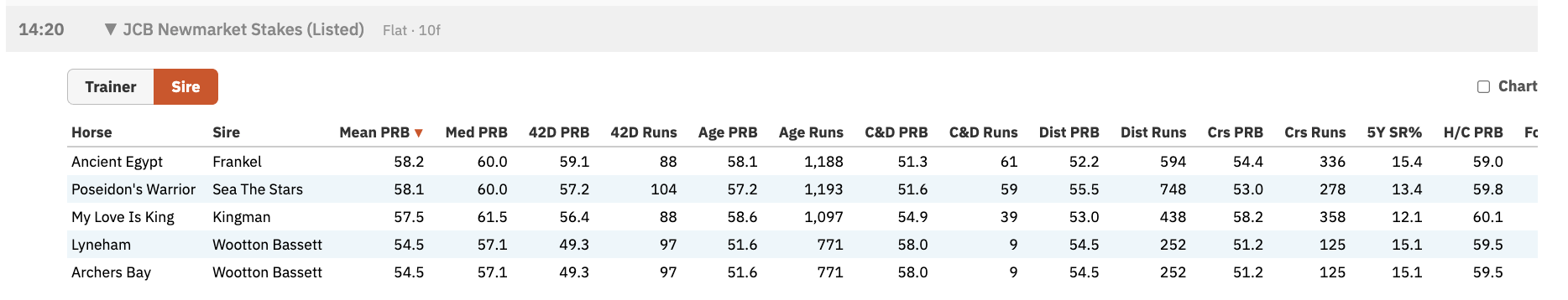
The charts then extend this by showing how those numbers behave in context.
Below the table, each sire has a set of box plots showing how their progeny have performed historically. See the screenshot for the charts (which can be toggled on or off from the main table):
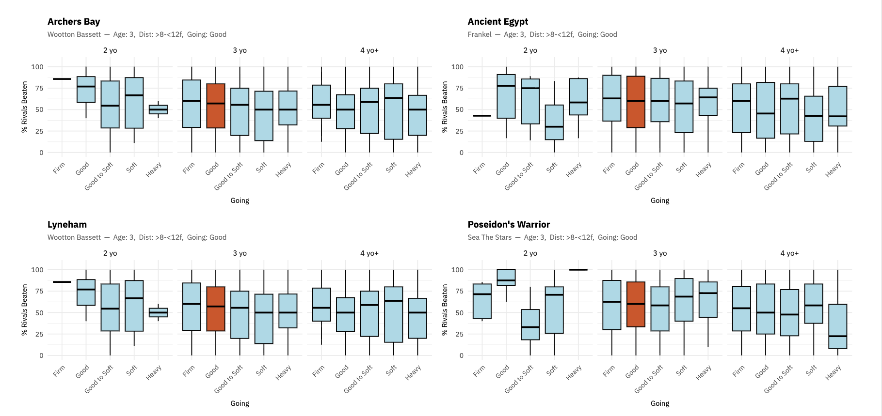
These are grouped by:
• Going
• Distance
Each box shows the distribution of % rivals beaten (PRB) for that sire under those conditions.
And then, for today’s race:
👉 the current runner is placed directly into that distribution
How To Read The Charts
You don’t need to overcomplicate it.
Each box gives you three useful pieces of information:
• The median line → typical level of performance
• The height of the box → how consistent that performance is
• The whiskers → how wide the range of outcomes is
The data on sires (particularly first or second season sires) is sometimes sparse, so interpret with care. However, as with this example, when the data is robust and there is a top rated performance, the signal can be very useful and gives us an interesting perspective that is often ignored.
In early season races, where the key question is often how well horses have trained from the previous year, the sire stats help assess the chances of all runners — and in this case highlighted the big-priced winner Ancient Egypt as top ranked. In answer to the question “Do progeny of Frankel train on from two to three?” the sire stats strongly support that view. The going, age and distance band stats answer the question: “Do progeny of Frankel perform under these conditions?” And the best thing – you get to see that relative to all the other runners in the race.
Used alongside trainer patterns, this helps build a more complete picture of how a race is likely to shape up. This is where the feature becomes practical — not just describing sire behaviour, but applying it directly to race analysis.
For now, Daily Sire Stats is available to all members, so you can explore the feature and see how it fits into your own approach.
Over time, it may become part of the subscriber-only offering, but for now it is there to be used and assessed in real conditions.
New: Daily Trainer Stats – How Today’s Runner Fits the Trainer’s Patterns
By colin on Monday, April 13th, 2026When we built Smartform back in 2007, the aim was to make it possible to work with racing data in a flexible way—combining variables, testing ideas, and building your own systems, apps and models.
Smartform still allows you to dig into the data—building your own variables and uncovering insights that aren’t immediately obvious.
But the reality is:
• Not everyone has the time
• Not everyone wants to code
• And even then, interpretation still matters.
A New Look at Trainer Patterns
One of the most interesting areas we’ve explored with Smartform over the years is trainer behaviour.
Patterns around:
• when horses are run
• how long they are rested
• what type of races they are placed in
…can all be measured, and over time they tend to be repeatable.
That’s where Daily Trainer Stats comes in. We’ve taken that approach and built a view that links the trainer’s historical patterns directly to today’s runner, using Smartform data and additional modelling layered on top.
What the Feature Shows
For every race, you are presented with:
• A sortable table of trainer statistics
• And a set of box plots underneath, specific to each trainer
The table is built from the Smartform dataset daily_trainers_insights, with all figures calculated on a “to date” basis—so they reflect exactly what would have been known at the time.
Each row gives you a structured view of the trainer’s performance:
• Mean / Median PRB (percentage of rivals beaten)
• Recent form (21D / 42D)
• Course, distance and C&D performance
• Handicap vs non-handicap performance
On its own, that already gives a solid overview.
But the key addition is how that information is extended in the charts.
The Box Plots: Adding visual context to the numbers
Below the table, each trainer has a set of box plots showing how their runners have performed historically.
These are grouped by:
• Age of the horse
• Days since last run (DSR)
Each box shows the distribution of % rivals beaten (PRB) for that trainer under those conditions.
And then, for today’s race:
👉 The current runner is placed directly into that distribution (highlighted in red)
This is the important step. Instead of looking at general trainer stats, you are looking at:
👉 How this trainer has performed with this type of horse, under these conditions, compared to all comparable runners from that trainer
How To Read The Charts
You don’t need to overcomplicate it.
Each box gives you three useful pieces of information:
• The median line → typical level of performance
• The height of the box → how consistent that performance is
• The whiskers → how wide the range of outcomes is
Then you look at where today’s runner sits within that.
In practical terms:
• A higher median suggests the trainer tends to outperform the field in that setup
• A more compressed box suggests those results are consistent
• A taller box or longer whiskers suggest more variability
What you are trying to judge is not just how good the trainer is—but how suitable today’s conditions are for that trainer.
A Worked Example: The First Race on Grand National Day
To show how this works in practice, we can look at the opening race on Grand National day, run at 12:45.
This was a Grade 1 novice chase—a race type where:
• the horses are still developing
• form is less complete
• and differences in trainer approach can be more revealing
Step 1: Shortlisting Candidates Using the Table
A straightforward way to begin is by sorting on 21-day PRB, to focus on trainers currently in form.
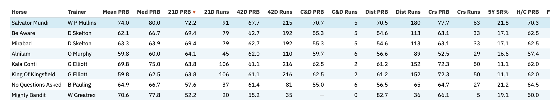
From the table (see screenshot), the top runners were:
• Salvator Mundi (W P Mullins)
• Mirabad (D Skelton)
• Be Aware (D Skelton)
That gives a manageable shortlist to examine in more detail.
Step 2: Looking at each horse’s profile
Within the charts for each race, you’ll find the individual horse profiles according to trainer patterns, in the case of our shortlist, some grainy screenshots below (see the app for full resolution!)
Rather than over-interpreting the charts ourselves, we presented them to ChatGPT with a simple description of the data and asked for an objective read. The result:
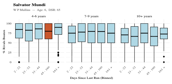
Salvator Mundi
From the chart:
• The distributions sit consistently above 50 PRB
• The median levels are strong across most segments
👉 This reflects a high baseline level of performance, regardless of exact conditions.
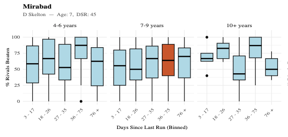
Mirabad
Looking at Mirabad’s highlighted position (orange box in chart):
• He sits in the 7–9 year-old group (column heading)
• With a mid-range break (DSR bin on x-axis)
In that segment:
• The box is relatively compressed
• The median is solid (mid-60 PRB range)
• The range of outcomes is not especially wide
👉 This indicates a consistent and repeatable level of performance under these conditions.
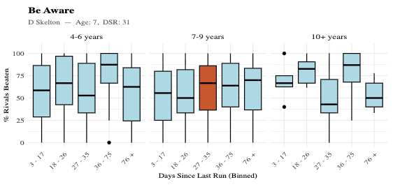
Be Aware
Also from the Skelton yard, but under slightly different conditions (see adjacent highlighted position):
• Similar overall level
• But the box in the relevant segment is taller
• With longer whiskers
👉 This suggests the trainer can produce strong results here, but with more variability in outcomes.
Step 3: Interpreting the Profiles Together
At this point, using both the table and charts, the prognosis for the race was as follows:
• Salvator Mundi
→ strongest overall profile
• Mirabad
→ consistent, well-aligned setup
• Be Aware
→ similar level, but less predictable
That gives a clear structure to the race before considering anything else.
The Race Result
• 1st: Mirabad (50/1)
• 2nd: Salvator Mundi (8/11)
• 3rd: Be Aware (10/1)
At the prices, Mirabad stood out as the runner whose profile was strongest relative to the market, at forecast odds of 33/1 (starting price 50/1).
What the example shows
The point here is not that the feature “found” a 50/1 winner.
It’s that, before the race:
• Mirabad was operating in a strong and consistent trainer setup (as shown in the chart)
• Be Aware, although similar in the table, had a more variable profile (taller box, longer whiskers)
• Salvator Mundi had the strongest overall profile, reflected in the market
The difference between Mirabad and Be Aware is particularly instructive.
From the table (top section), they appear quite similar.
From the charts (bottom section), you can see:
• one sits in a more stable, repeatable performance zone
• the other in a wider, less predictable range
That distinction is not obvious from summary statistics alone.
Where This Fits
All of this is built from the same Smartform data.
If you want to go further—build your own metrics, test ideas, or explore different angles—Smartform enables that.
What Daily Trainer Stats does is take one part of that work and present it in a way that can be used quickly, across every race.
Final Note
Trainer patterns are only one part of the picture.
You still need to consider:
• the horse itself
• the opposition
• a broader set of historical statistics, all of which are available in Smartform
But being able to see trainer angles very clearly as a unique starting point is a useful angle, in particular whether a runner is operating in a situation where the trainer has historically performed well.
For now, Daily Trainer Stats is available to all members, so you can explore the feature and see how it fits into your own approach.
Over time, it may become part of the subscriber only offerings, but for now it is there to be used and assessed in real conditions.
New: daily_sires_insights Table Now in Smartform
By colin on Monday, September 1st, 2025Following on from our recent releases of daily_trainers_insights and daily_jockeys_insights, we’re pleased to announce the addition of a new insights table to Smartform: daily_sires_insights.
This new table contains engineered statistics for every runner since March 2008, summarising the historic performance of each horse’s sire under a wide range of conditions. With over 2.3 million rows and 40+ variables, daily_sires_insights lets you query:
- Percentage of Rivals Beaten (PRB) and strike rate
- Split by course, distance, race type, race code, age group, and handicap status
- Across three timeframes: last 5 years, 42 days, and 21 days
- For each day in the database — fully backtestable and forward-compatible
As with other Smartform daily insights tables, the values are rolled up to the date of the race (i.e. no leakage from future performance), making it ideal for both live betting systems and historical model building.
While the table can power complex backtesting pipelines or machine learning models, it also offers immediate value even for simple queries.
For example, here’s a single race from the weekend at Sandown (14:25) where we used the rt_5Y_course_prb variable to rank the sires of each runner by their average performance at the course over the last five years. The top-ranked sire was flagged automatically from the data, and for our cherry-picked example that horse went on to win at 14/1.
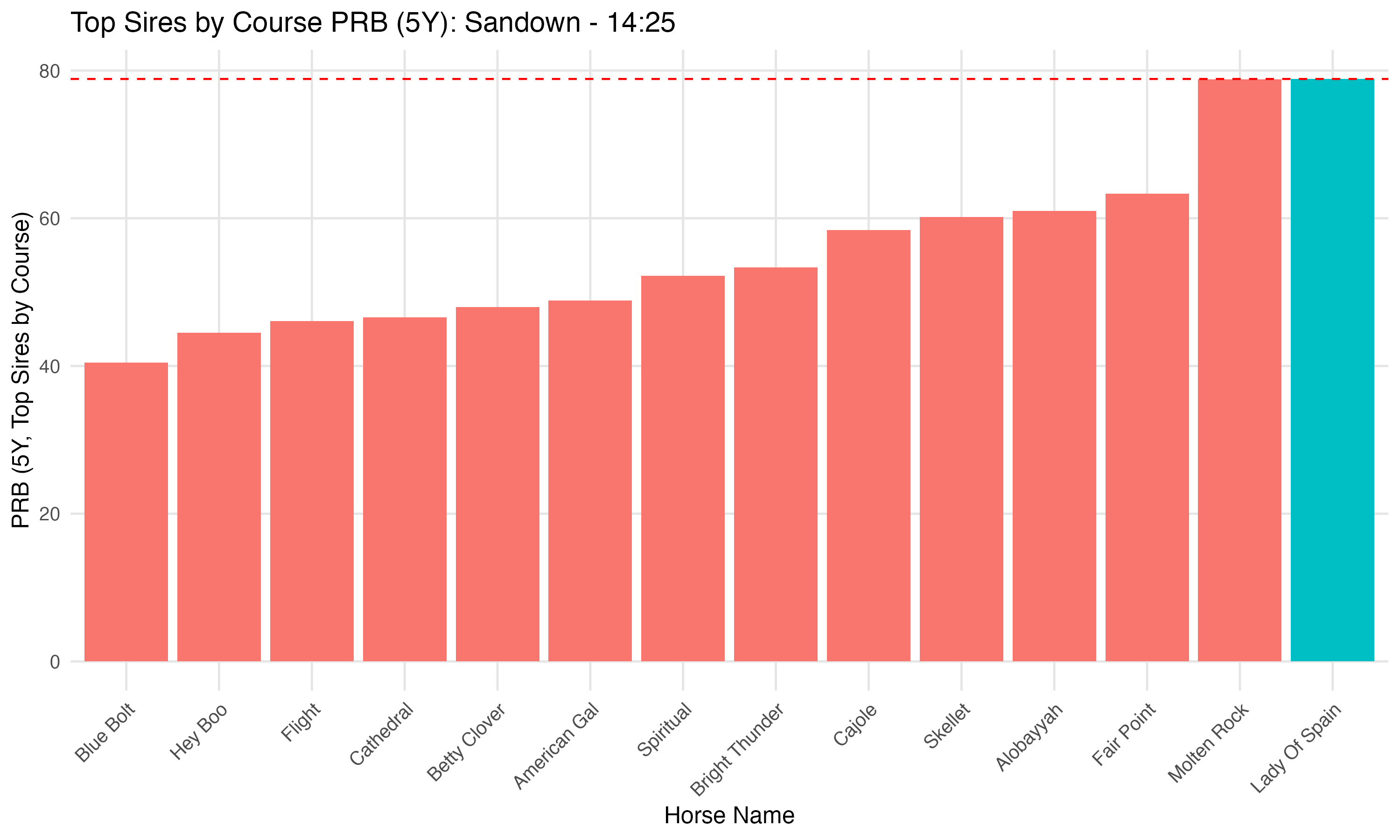
This query took just a few lines of SQL to join the daily_sires_insights table with the runners for the race and calculate the rankings:
SELECT
r.horse_name,
s.prb_5yr_by_course
FROM
daily_runners r
JOIN
daily_sires_insights s
ON r.meeting_date = s.meeting_date AND r.horse_name = s.horse_name
WHERE
r.meeting_date = '2025-08-31'
AND r.course = 'Sandown'
AND r.race_time = '14:25'
ORDER BY
s.prb_5yr_by_course DESC;
This is just one of many ways to use the table — in fact, every runner in every race comes with this level of insight now built in. So whether you’re looking to test broader breeding strategies or just want a quick read on today’s runners, this table has you covered.
Smartform subscribers can now download the new daily_sires_insights dataset by visiting the downloads section of the site once logged in. You can view the full schema here, including all field definitions and update schedule.
As always, if you have any questions or suggestions, feel free to get in touch.
Enjoy!
Calculating price movements
By Nick Franks on Thursday, May 15th, 2025In my previous blog post, I explained how meaningful odds can be extracted from the betting_text column in the historic_runners tables. We will now discuss how these odds can be converted into a decimal price and compared again with the starting price to produce a price movement for each runner in a race.
The SQL script below builds a table called all_prev_race_price_movements. It holds information about each horse’s latest race for a specific type of race (such as turf, all-weather, etc.) and, where possible, details from the horse’s previous race of the same type.
The script then works out how the betting odds changed between the two races — basically, tracking if a horse was backed or drifted in the market.
The script returns not just the price movement but other pieces of useful data for the current and previous runs. Eg. finish_position, position_in_betting, unfinished, distance_won, distance_beaten, etc. (This data will be useful in the next blog post, where we will show how the table created can be use to analyse the data further).
Takeaways from the full SQL script below:
This setup allows you to:
- See how a horse’s market position changed from one race to the next.
- Spot if a horse was heavily backed (shortened in price) or was not fancied (ie. the price drifted).
- Compare races of the same type only, so the analysis is consistent.
Step-by-Step Breakdown
1. RankedRaces
- This section links together races and runners.
- It gives each race a ranking within its race type, with the most recent races ranked highest.
2. LastRaceTimes
- This picks out the most recent race for each race type.
- It helps make sure we only look at races up to the latest one — anything in the future gets ignored.
3. FilteredRaces
This is the main bit of the logic.
- It filters out races that happened after the most recent one.
- It ranks each runner’s races within that race type — so we can tell which was most recent run, which was next most recent run, and so on.
- It fetches details like the starting price, where the horse finished, etc.
- It also attempts to extract the opening odds from the betting summary text ( as covered in my previous blog post).
- It calculates a percentage chance (ie. probability) implied by the starting price.
4. ProcessedRaces
- Adds a calculation to convert the opening odds into a percentage.
- This allows us to compare the market expectation before the race with the actual SP (starting price).
Final Output (SELECT Statement)
The final section:
- Focuses on the most recent race for each horse and race type.
- Tries to link it to the previous race of the same type for the same horse.
- If no such race exists, the previous race columns are just left empty (NULL).
- Works out the percentage change from the opening price to the starting price — this shows whether the horse was backed in (price dropped) or drifted (price lengthened).
- The whole code below has the following criteria to return results for horses in races in the last 3 months, this can be changed as desired.
AND curr.scheduled_time >= DATE_SUB(CURRENT_DATE, INTERVAL 3 MONTH)The results of this SQL can been seen by running a simple select:
SELECT * FROM all_prev_race_price_movements;Full SQL Script:
DROP TABLE IF EXISTS all_prev_race_price_movements;
CREATE TABLE all_prev_race_price_movements AS

WITH RankedRaces AS (
    SELECT
        hr.scheduled_time,
        hru.runner_id,
        hr.race_id,
        hr.race_type_id,
        hr.handicap,
        hru.starting_price,
        hru.starting_price_decimal,
        hru.position_in_betting,
        hru.finish_position,
        hru.unfinished,
        hru.distance_won,
        hru.distance_beaten,
        hru.official_rating,
        hru.betting_text,
        RANK() OVER (PARTITION BY hr.race_type_id ORDER BY hr.scheduled_time DESC) AS race_type_rank
    FROM historic_races hr
    JOIN historic_runners hru USING (race_id)
), LastRaceTimes AS (
    SELECT
        race_type_id,
        MAX(scheduled_time) AS last_race_time
    FROM RankedRaces
    WHERE race_type_rank = 1
    GROUP BY race_type_id
), FilteredRaces AS (
    SELECT
        rr.scheduled_time,
        rr.runner_id,
        rr.race_id,
        rr.race_type_id,
        rr.handicap,
        rr.official_rating,
        rr.starting_price AS previous_starting_price,
        rr.starting_price_decimal AS previous_starting_price_decimal,
        rr.position_in_betting AS previous_position_in_betting,
        rr.finish_position AS previous_finish_position,
        rr.unfinished AS previous_unfinished,
        rr.distance_beaten AS previous_distance_won,
        rr.distance_beaten AS previous_distance_beaten,
        rr.official_rating AS previous_official_rating,
        rr.handicap AS previous_handicap,
        rr.betting_text AS previous_betting_text,

        -- Parse odds string
        IFNULL(
            REPLACE(
                REGEXP_SUBSTR(
                    rr.betting_text,
                    '(?<=op )\\d{1,3}/\\d{1,3}|(?<=tchd )\\d{1,3}/\\d{1,3}|(?<=op )Evens|(?<=tchd )Evens'
                ),
                'Evens',
                '1/1'
            ),
            '0/0'
        ) AS derived_previous_odds,

        -- Cast to prevent divide by zero, using DECIMAL to avoid FLOAT deprecation
        CASE
            WHEN rr.starting_price_decimal > 0 THEN
                CAST(CAST(100 AS DECIMAL(20,10)) / CAST(rr.starting_price_decimal AS DECIMAL(20,10)) AS DECIMAL(20,10))
            ELSE NULL
        END AS previous_SP_pct,

        ROW_NUMBER() OVER (PARTITION BY rr.runner_id, rr.race_type_id ORDER BY rr.scheduled_time DESC) AS race_rank
    FROM RankedRaces rr
    JOIN LastRaceTimes lrt ON rr.race_type_id = lrt.race_type_id
    WHERE rr.scheduled_time <= lrt.last_race_time
), ProcessedRaces AS (
    SELECT *,
        -- Convert odds string to decimal price percentage using DECIMAL
        CASE
            WHEN REGEXP_LIKE(derived_previous_odds, '\\d+/\\d+') AND
                 CAST(SUBSTRING_INDEX(derived_previous_odds, '/', -1) AS DECIMAL(20,10)) > 0
            THEN CAST(
                CAST(100 AS DECIMAL(20,10)) / (
                    CAST(SUBSTRING_INDEX(derived_previous_odds, '/', 1) AS DECIMAL(20,10)) /
                    CAST(SUBSTRING_INDEX(derived_previous_odds, '/', -1) AS DECIMAL(20,10)) +
                    CAST(1 AS DECIMAL(20,10))
                )
                AS DECIMAL(20,10)
            )
            ELSE NULL
        END AS previous_opening_price_pct
    FROM FilteredRaces
)
SELECT
    curr.runner_id,
    curr.race_type_id,
    curr.scheduled_time AS current_race_time,
    curr.race_id AS current_race_id,
    curr.handicap AS current_handicap,
    curr.official_rating AS current_official_rating,
    prev.scheduled_time AS previous_race_time,
    prev.race_id AS previous_race_id,
    prev.previous_starting_price,
    prev.previous_starting_price_decimal,
    prev.previous_position_in_betting,
    prev.previous_finish_position,
    prev.previous_unfinished,
    prev.previous_distance_won,
    prev.previous_distance_beaten,
    prev.previous_official_rating,
    prev.previous_handicap,
    prev.previous_betting_text,
    prev.derived_previous_odds,
    prev.previous_SP_pct,
    prev.previous_opening_price_pct,


-- Safe percentage movement calc using DECIMAL only
CASE
    WHEN prev.previous_opening_price_pct > 0 THEN
        CAST((
            (CAST(prev.previous_SP_pct AS DECIMAL(20,10)) - CAST(prev.previous_opening_price_pct AS DECIMAL(20,10)))
            / CAST(prev.previous_opening_price_pct AS DECIMAL(20,10))
        ) * CAST(100 AS DECIMAL(20,10)) AS DECIMAL(20,10))
    ELSE NULL
END AS previous_price_movement
FROM ProcessedRaces curr
LEFT JOIN ProcessedRaces prev
    ON curr.runner_id = prev.runner_id
    AND curr.race_type_id = prev.race_type_id
    AND prev.race_rank = curr.race_rank + 1
WHERE curr.race_rank = 1
AND curr.scheduled_time >= DATE_SUB(CURRENT_DATE, INTERVAL 3 MONTH)
ORDER BY curr.race_type_id, curr.runner_id;
Extracting useful data from the betting string
By Nick Franks on Sunday, May 11th, 2025This post comes as a result of thinking about ways to calculate the price movements of horses, from the opening show to the SP. The opening show and other price movements aren’t currently available in Smartform as separate fields, however the opening show and other price movements are contained within the betting_text column in the historic_runners and historic_runners_beta tables, stored as a text string.
The question is how to split out the data. After a number of experiments, I came up with the following SQL to derive a usable price to go to work with. In my next post I will describe how to convert this to a decimal price and calculate the price movement from the opening show to starting price.
IFNULL(
     REPLACE(
         REGEXP_SUBSTR(
             betting_text,
             '(?<=op )\d{1,3}/\d{1,3}|(?<=tchd )\d{1,3}/\d{1,3}|(?<=op )Evens|(?<=tchd )Evens'
         ),
         'Evens',
         '1/1'
     ),
     '0/0'
 ) AS derived_previous_odds
The above code looks into the string field called betting_text and tries to find the previous odds of a horse from the point at which the betting shows open on course before any given race
Here’s what each part does:
REGEXP_SUBSTR(...):
This searches the text for the first match of one of the following patterns:- A fraction like
5/2,11/8, etc. that appears after the word “op “ (short for “opened at”) - A fraction that appears after the word “tchd “ (short for “touched”)
- The word
"Evens"(which means 1/1 odds) after either “op ” or “tchd “
- A fraction like
REPLACE(..., 'Evens', '1/1'):
If the match found was"Evens", this replaces it with"1/1"to standardize it into fractional format.IFNULL(..., '0/0'):
If nothing matched (i.e., there were no odds found in the text), it returns'0/0'instead of null.
Examples
betting_text = "op 5/1 tchd 6/1"
- Match found:
"5/1"(after"op ") - Replacement: None
- Final result:
"5/1"
betting_text: "op Evens tchd 11/10"
- Match found:
"Evens"(after"op ") - Replacement:
"Evens"→"1/1" - Final result:
"1/1"
betting_text = "op 85/40 tchd 2/1"
- Match found:
"85/40"(after"op ") - Replacement: None
- Final result:
"85/40"
betting_text = "tchd 30/100 op 4/5"
- Match found:
"30/100"(after"tchd ") - Replacement: None
- Final result:
"30/100"
betting_text = "non-runner, withdrawn at start"
- Match found: None (no “op” or “tchd” with odds or “Evens”)
- Replacement: Not applicable
- Final result:
"0/0"(default value when nothing matches)
New: daily_jockeys_insights comes to Smartform
By colin on Tuesday, December 10th, 2024Hot on the heels of our post about the new daily trainers insights variables available to Smartform users, we’re pleased to announce the addition of a new corresponding table for jockeys: daily_jockeys_insights.
You can view the new schema and Smartform users can download all the data (all 2.3 million new rows) following the instructions under “Downloading the data” here.
The new table follows the format and category types designed for daily_trainers_insights, but instead curating statistics for all daily races and runners since March 2008 according to jockey performance. All the details are in the schemas, and the previous blog article on trainer_insights holds true but this time for the riders. Rather than restate the high level details in this blog post, we will instead show what it is possible to achieve using one of the unique fields in the table.
In this example, presented below, we joined the daily_jockeys_insights table to the daily_runners_insights table for all yesterday’s racing at Wolverhampton, removing non-runners, and focussed on the percentage rivals beaten (PRB) statistics for each jockey riding in each race, but over the past 5 years using the values automatically generated in the new table. The particular PRB statistic we used comes with a twist, however, in that it considers the performance of each jockey according to the handicap status in the race in which the jockey is competing. In other words, each PRB figure is applied to the jockey’s performance in handicaps or non-handicaps – and the 5 year PRB figure for all the jockeys rides up to but not including the race is presented – according to the handicap status of the current race in question. Note that each comparison, as presented below, can be generated prior to racing, and you can also interrogate previous day’s statistics by entering the relevant meeting date. We then wrote a graphics script to plot the runners in each race, showing each jockey below the runner name, and highlighting the runner and jockey in bold which has the highest PRB statistic within the context of the race. The red dashed line shows the level of the PRB for the highest rated jockey within each race. Below are the results.

Finally, let’s look at the results for each race by querying Smartform on the highlighted runners and jockeys above.
| Course | Race Time | Horse | Jockey | Result | Starting Price |
| Wolverhampton | 16.15 | Lewis Barnes | Kaiya Fraser | 2 | 9/4 |
| Wolverhampton | 16.45 | Diomed Spirit | Marco Ghiani | 3 | 7/1 |
| Wolverhampton | 17.15 | Onslow Gardens | Tyrese Cameron | 4 | 11/8 |
| Wolverhampton | 17.45 | Bear Rock | R Kingscote | 2 | 66/1 |
| Wolverhampton | 18.15 | Windsor Pass | Kaiya Fraser | 5 | 4/1 |
| Wolverhampton | 18.45 | Eagle Day | R Kingscote | 1 | 15/2 |
| Wolverhampton | 19.15 | Moon Over The Sea | Jack Doughty | 5 | 9/2 |
| Wolverhampton | 19.45 | Khangai | Hector Crouch | 3 | 5/4 |
| Wolverhampton | 20.15 | Alfheim | Tommie Jakes | 1 | 11/4 |
Given we are using just one variable from the new table, these are, we hope you will agree, interesting results: 2 well priced winners, with 4 placed horses also at interesting prices, and 3 losers.
What is particularly interesting about using the “by handicap status” condition is that whilst you do get some repeats (as with Richard Kingscote and Kaiya Fraser, each qualifying in 2 races, above), one jockey that has good statistics does not dominate the whole meeting’s statistics. This can happen with (for example) course statistics by jockey. Where you do want to highlight “the best” jockey at a course, this also has its uses, and this too is available in the new table, along with 40+ other variables. Enjoy!
New: daily_trainers_insights now available in Smartform
By colin on Tuesday, December 3rd, 2024We’ve added a new database table to Smartform. Over 2.29 million new rows of data and 48 columns, representing all daily runners since the daily* tables started in March 2008 (for both Flat and Jumps racing), with every runner mapped to the historic performance of the trainer responsible, with statistics aggregated for all the trainer’s runners over the previous 5 years to that run, the previous 42 days and the previous 21 days to the run, covering statistics for race type performance, race code performance, performance at distance, course, in handicaps, by age of horse and much more. Thus you can track short and long term performance for each trainer by a number of different metrics.
With Smartform, you can of course create your own statistics for historical trainer performance, and there are a practically infinite number of possibilities in addition to those included in the default table. You can see some old blog posts showing how to do this on a daily basis, here and here. However we appreciate that many users do not want to program their own statistics, maintain the data, or would like a convenient baseline of performance statistics in addition to their own work that can be queried as a table at will. For all these use cases, daily_trainers_insights is now available and can be downloaded here. See the link at the last section of the page once you are logged in to the site as a subscriber, or sign up for access if you want to become a subscriber or rejoin.
All the statistics in these tables have been engineered from the data in the Smartform database to provide insight on top of the raw data, from standard win and place strike rates to more granular variables like average number of horses beaten according to distance, course, course and distance, age, handicap, race_type and race_code. You can see the full table definition and an explanation of all the variables here.
There’s more that you can do with the new table than we have space to cover here, but we’ll be writing more about different use cases for the new table over the coming weeks. To whet the appetite, here’s a graph we threw together for today’s racing that shows off 3 of the new statistics for short, medium and long term performance statistics by percentage of rivals beaten. So each horse in each race has 3 bars for the 21 day, 42 day and 5 year strike rate by race code.
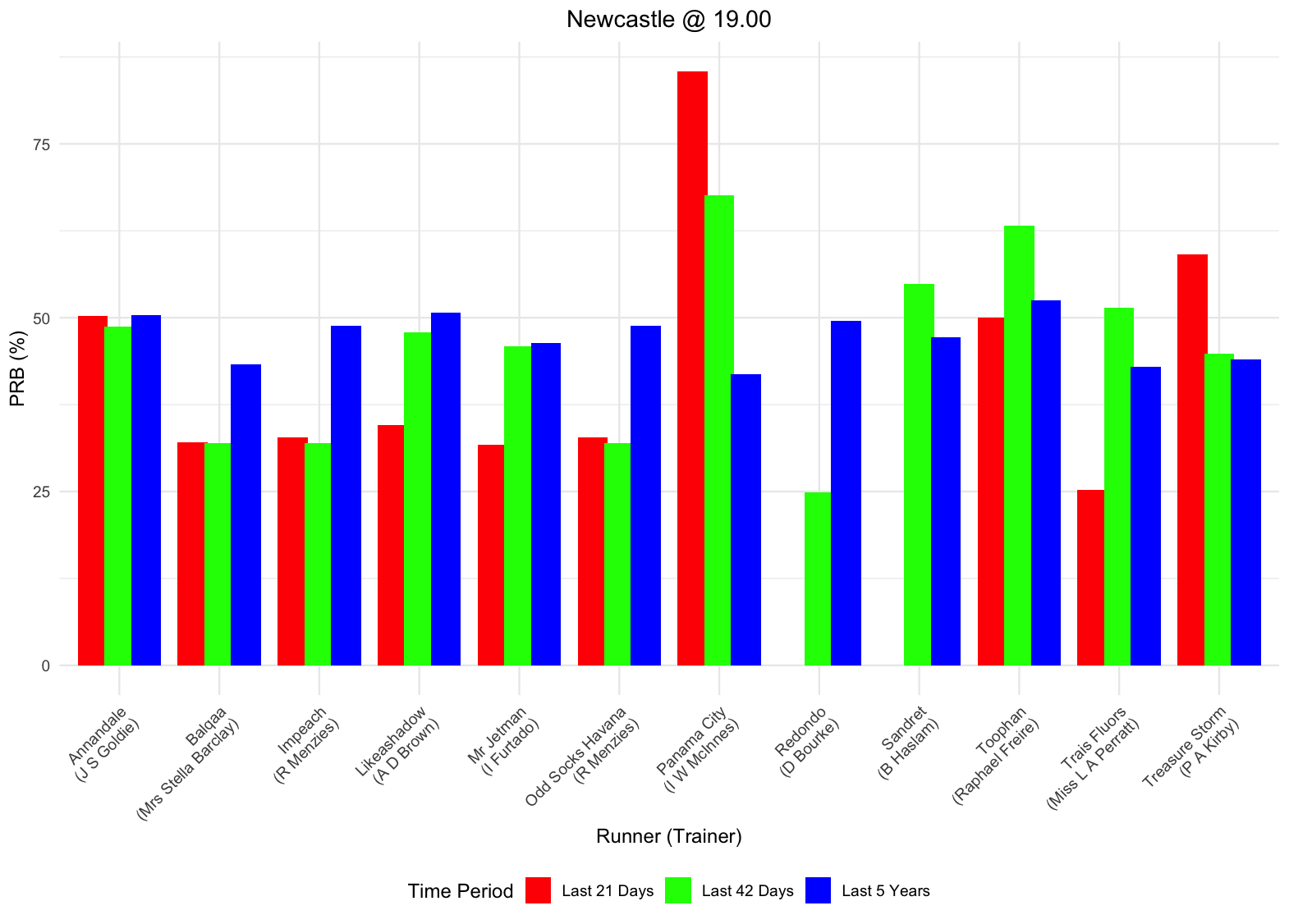
Standout short term PRB statistics for the trainer of Panama City – which of course went on to win!
Unlike most of the other tables in Smartform, there is no “historic” version of this table, since all the historic statistics for each trainer are available for every day since March 2008, as it corresponds exactly to the daily_runners_beta and daily_runners table, which also run from March 2008. However, this table contains fields that are calculated based on all previous races of the same type to give you an indication of the trainer’s historic performance and updates for every day. For example, in a flat all weather handicap race today, you will be able to find statistics relating to the trainer’s previous 5 year strike rate for all runners in flat all weather handicaps.
Since it is updated for each day you have all the statistics you need to make an informed judgement about a trainer’s historic performance for runners under today’s conditions. Similarly, you can go back in time to any previous day’s racing to find the statistics that were pertinent to the trainer’s historic performance at that time.
Each variable has been painstakingly tested to ensure that the correct previous information is provided on a “to date” basis for each runner at the time of entry in the historic database without taking into account the result of the upcoming run. This means systems backtesting and modelling use cases are all valid with this dataset.
We hope you enjoy using daily_trainers_insights as much as we have enjoyed crafting it and writing about it. If you have questions about the new table, please do not hesitate to get in touch.
Nine (9) new fields for Smartform
By colin on Friday, November 15th, 2024We’ve just updated daily_runners_insights and historic_runners_insights. These tables already contain numerous utility or short cut fields that mean users can avoid lengthy queries on each runner in a race to find details on their previous performances and instead query the race runners and have all that data in a single row, for immediate analysis.
The recent updates fill out those details for a few variables that were previously missing for the previous few races, such as the course last time out, the race type and the jockey. We have jockey changes, course changes and race type changes – all themselves useful as rapid indicators for differences since the last run, but now we can be more specific. Check out the table schemas, linked above, for full details.
Stay tuned for a number of (even more) exciting additions to Smartform in the coming weeks!
Roger Fell : More trainer_ids to merge
By Henry Young on Thursday, October 24th, 2024Last year I wrote about Mark Johnston partnering with then handing over his trainers license to his son Charlie and the impact this had on Smartform’s trainer_id. Those of us who like to aggregate data by trainer_id, for example to generate trainer strike rates, might wish to acknowledge that the Johnstons’ yard and training methods remained substantially the same through this handover of the reins (pun intended) by merging all the various trainer_id values together into one. Well, it’s happened again …
Roger Fell’s yard has been going through some drama with the addition of Sean Murray as a partner on the trainer’s license. However Sean’s name has more recently disappeared from the license. Roger Fell continues in his own right, an example to all of us, still working at age 70. One consequence is that Smartform’s data provider has changed trainer_id, but only when Sean Murray was dropped, not when he was added. We can observe this with the following query:
select distinct trainer_id, trainer_name from historic_runners_beta where trainer_name like "%Fell%";
+------------+--------------------------+
| trainer_id | trainer_name             |
+------------+--------------------------+
|       1220 | R Fell                   |
...
|     128659 | Roger Fell               |
|     128659 | Roger Fell & Sean Murray |
|     161959 | Roger Fell               |
+------------+--------------------------+
5 rows in set (6.30 sec)
Note there is an unrelated trainer whose name contains “Fell” whom I have removed from the results table for clarity.
The first thing we see is that when Sean joined the trainer license, the trainer_id remained the same. But when Sean left the license, a new trainer_id was created for Roger on his own. If you take the view that nothing significant has changed about how the yard is run, the staff, the training methods, etc, you may prefer to see results from all four Fell licenses under a single trainer_id. This can be done with the following SQL script:
SET SQL_SAFE_UPDATES = 0;
UPDATE historic_runners_beta SET trainer_id = 161959 WHERE trainer_name = "R Fell";
UPDATE historic_runners_beta SET trainer_id = 161959 WHERE trainer_name = "Roger Fell";
UPDATE historic_runners_beta SET trainer_id = 161959 WHERE trainer_name = "M Johnston";
SET SQL_SAFE_UPDATES = 1;
Note that here we are using the newest trainer_id to tag all past results. This means the modification is a one-time deal and all future runners/races will continue to use the same trainer_id. If we had used any of the older trainer_id values, we would have to apply the fix script every day, which would be far less convenient.
This concept is easily extended to other trainer changes. For example, if your would like aggregated stats for the partnership between Rachel Cook and John Bridger to be merged with John’s longer standing stats, you can add the following to your script:
UPDATE historic_runners_beta SET trainer_id = 157470 WHERE trainer_name = "J J Bridger";If you find there are other trainer name changes that have resulted in a new trainer_id which you would prefer to see merged, you can apply similar techniques.
If you know of other cases of trainer name changes which represent a continuation of substantially the same yard, please feel free to comment …