
Archive for May, 2018
O’Brien and Moore in Group Races – Scatterplots with R
Saturday, May 26th, 2018Last week we looked at the performance of Aiden O’Brien trained horses running in Group races. As an exercise for the reader it was suggested to look at the combination of both Aiden O’Brien and Ryan Moore in Group races. The result was that this combination showed an overall profit since 2007.
The R code was provided at the end of the article and this will be used as the starting point today. Rather than show all code during the article, it is assumed the reader can now connect to the Smartform MySQL database and retrieve basic data. Nonetheless, the full R code for today’s investigations will be provided at the end of the article.
Starting with O’Brien and Moore in all Group races since 2007.
# Variable smartform_results contains data retrieved from the Smartform MySQL database
# Filter SQL results for flat races only
flat_races_only <- dplyr::filter(smartform_results,
                                 race_type_id == 12 |
                                   race_type_id == 15)
# Filter for Group races only
group_races_only <- dplyr::filter(flat_races_only,
                                  group_race == 1 |
                                    group_race == 2 |
                                    group_race == 3 )

# Filter for Aiden O'Brien runners only
obrien_group_races_only <- dplyr::filter(group_races_only,
                                         grepl("A P O'Brien", trainer_name))

# Remove non-runners
obrien_group_races_only <- dplyr::filter(obrien_group_races_only, !is.na(finish_position))

# Filter for Ryan Moore rides only
obrien_moore_group_races_only <- dplyr::filter(obrien_group_races_only,
                                               grepl("R L Moore", jockey_name))

# Calculate Profit and Loss
obrien_moore_cumulative <- cumsum(
  ifelse(obrien_moore_group_races_only$finish_position == 1, (obrien_moore_group_races_only$starting_price_decimal-1),-1)
)

obrien_moore_group_races_only$cumulative <- obrien_moore_cumulative

# Convert meeting_date columns to Date type
obrien_moore_group_races_only$meeting_date <- as.Date(obrien_moore_group_races_only$meeting_date)

# Plot the results
ggplot(data=obrien_moore_group_races_only, aes(x=meeting_date, y=cumulative, group=1)) +
  geom_line(colour="blue", lwd=0.7) +
  scale_x_date(labels = date_format("%Y-%m-%d"), date_breaks="6 months") +
  theme_tufte(base_family="serif", base_size = 14) +
  geom_rangeframe() +
  theme(axis.text.x = element_text(angle = 45, hjust = 1),
        panel.grid.major.x = element_line(color = "grey80"),
        panel.grid.major.y = element_line(color = "grey80"))
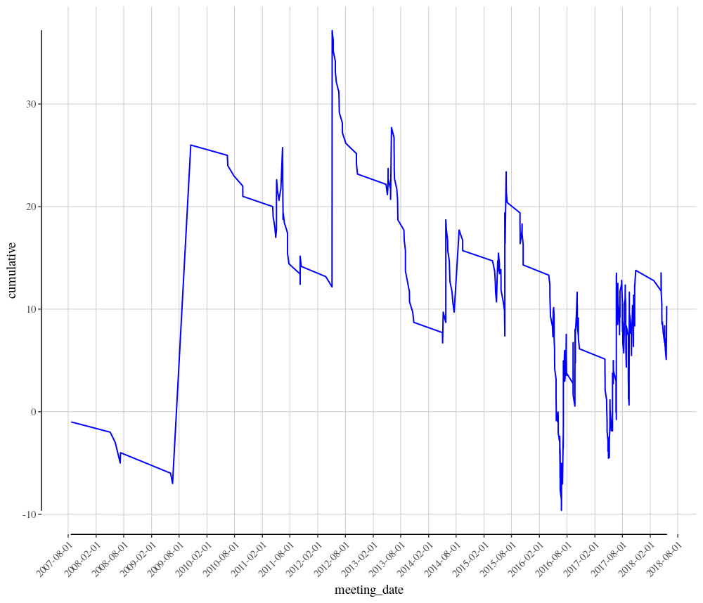
The chart and profit and loss calculations indicate a small profit of 10.31 for a one unit stake across all 377 runners in the dataset. Decent enough, however, we should always ask if this is the full story.
One way of investigating further is to create a scatter plot of the Starting Price for all O’Brien and Moore winners. The ggplot library is again used for this. There are many very powerful features of this charting tool and a wide number of tutorials available online.
# Filter for winners only
obrien_moore_group_races_winners_only <- dplyr::filter(obrien_moore_group_races_only,
                                                       finish_position == 1)

# Scatter plot of winning prices for all O'Brien and Moore winners
ggplot(obrien_moore_group_races_winners_only , aes(x=meeting_date, y=starting_price_decimal)) +
  geom_point(colour="blue") +
  scale_x_date(labels = date_format("%Y-%m-%d"), date_breaks="6 months") +
  theme_tufte(base_family="serif", base_size = 14) +
  theme(axis.text.x = element_text(angle = 45, hjust = 1),
        panel.grid.major.x = element_line(color = "grey80"),
        panel.grid.major.y = element_line(color = "grey80")) +
  geom_smooth(method=loess,
              color="darkred")
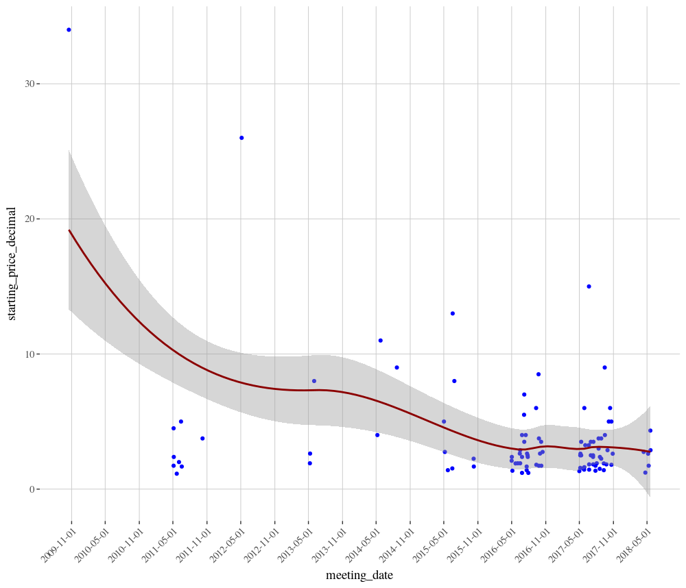
This very interesting chart includes a loess regression line with confidence intervals. The line indicates that the price of O’Brien and Moore winners has been reducing over time, although it also appears that the confidence interval narrows (a good thing!) as the number of rides increases. The slight increase in confidence interval in 2018 is due to the fact the season is not yet half completed and the overall number of runners for this combination is low so far this year.
The chart also clearly shows that the overall Profit and Loss is probably skewed by the big priced winners in 2009 and 2012. If these two rides were removed, the combination would show an overall large loss.
We could also plot every individual runner for this combination, with a separate regression line for both winners and all other runners. In the chart below, winners are the blue points and all other runners are orange.
# Scatter plot of winning prices for all O'Brien and Moore runners
ggplot(obrien_moore_group_races_only , aes(x=meeting_date, y=starting_price_decimal, color=finish_position == 1)) +
  geom_point() +
  scale_x_date(labels = date_format("%Y-%m-%d"),
               date_breaks="12 months") +
  scale_y_continuous(breaks= seq(0,35,by=2)) +
  theme_tufte(base_family="serif",
              base_size = 14) +
  theme(axis.text.x = element_text(angle = 45, hjust = 1),
        panel.grid.major.x = element_line(color = "grey80"),
        panel.grid.major.y = element_line(color = "grey80"),
        legend.position="top") +
  scale_color_manual(values=c("#FF9933","#000CCC")) +
  geom_smooth(method=lm, se=FALSE, fullrange=TRUE)
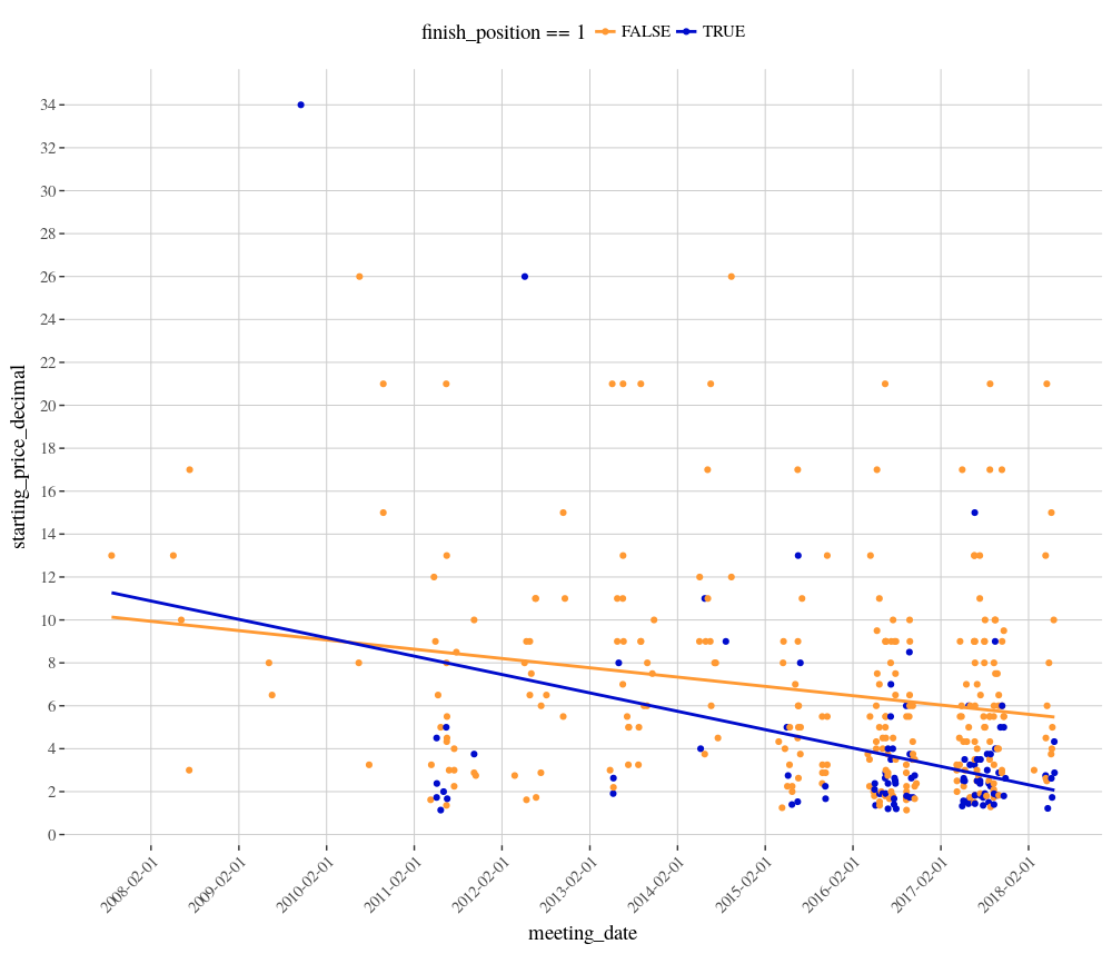
This chart shows that there are tight clusters of winners and runners in 2016 and 2017. We can also see that the starting price of winners has been contracting faster than the overall price of all starters for this combination. As bettors, we should always keep in mind the value proposition of a bet.
Next, we could filter the data and examine just runners from the 2016 season onwards, with a starting price of less than 4.00.
# Filter the data for starters at an SP of less than 4.0 and since 2016 only
obrien_moore_group_races_only_price_filter <- dplyr::filter(obrien_moore_group_races_only,
                                                            starting_price_decimal <= 4.0 &
                                                              meeting_date >= "2016-01-01")

# Calcualte profit and loss
obrien_moore_cumulative <- cumsum(
  ifelse(obrien_moore_group_races_only_price_filter$finish_position == 1, (obrien_moore_group_races_only_price_filter$starting_price_decimal-1),-1)
)

obrien_moore_group_races_only_price_filter$cumulative <- obrien_moore_cumulative

# Plot the results as a line chart
ggplot(data=obrien_moore_group_races_only_price_filter, aes(x=meeting_date, y=cumulative, group=1)) +
  geom_line(colour="blue", lwd=0.7) +
  scale_x_date(labels = date_format("%Y-%m-%d"), date_breaks="6 months") +
  theme_tufte(base_family="serif", base_size = 14) +
  geom_rangeframe() +
  theme(axis.text.x = element_text(angle = 45, hjust = 1),
        panel.grid.major.x = element_line(color = "grey80"),
        panel.grid.major.y = element_line(color = "grey80"))

# Calculate strike rate
winners_only <- nrow(dplyr::filter(obrien_moore_group_races_only_price_filter,
                                    finish_position == 1))

runners <- nrow(obrien_moore_group_races_only_price_filter)

strike_rate <- (winners_only / runners) * 100
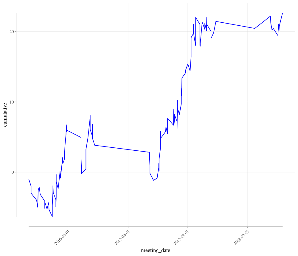
We now have a very healthy 22.67 profit from 133 runners over the last two seasons, with a strike rate of 49.62%. This seems like a quite nice angle into Group races where Aiden O’Brien has a horse ridden by Ryan Moore.
The chart shows that 2016 was a bit slow to begin with, but than picked up nicely from around June onwards. However, 2017 was a very strong year. This year, 2018, seems to be off to a decent start.
There are many other angles which could be investigated. For example, we could filter for:
- Group 1 races only
- Odds on runners only
- Odds between 2.0 and 4.0
- Odds less than 10.0 only
- A distance filter
- A UK vs Ireland scatter chart and filter
There are many, many different ways of investigating further.
Today’s races includes the Irish 2000 Guineas at the Curragh, as well as some other Group races on the same card. Are there any O’Brien and Moore qualifiers?
There are three qualifying horses – US Navy Flag in the Irish 2000 Guineas, Merchant Navy in the Group 2 Greenland Stakes and Hydrangea in the Group 2 Lanwades Stud Stakes, all at prices less than 3/1.
Are all three worth a bet? There’s always something else to consider. Why did Ryan Moore’s number of rides and winners increase markedly from 2016 onwards? In March 2016 Joseph O’Brien announced his retirement from race riding. Ryan Moore most likely then picked up a number of high quality rides which would have otherwise gone to Joseph.
In the 2000 Guineas at Newmarket a few weeks ago, another of Aiden O’Brien’s sons, Donnacha, had a winning ride on Saxon Warrior. This may have only been because Moore was otherwise engaged for Ballydoyle at the Kentucky Derby. What are the current internal dynamics at the stable now? Has Donnacha’s success elevated him in the pecking order?
Donnacha O’Brien rides Gustav Klimt in today’s 2000 Irish Guineas. How important is this race for the stable? Is it an opportunity for Donnacha to ride another Group 1 winner? Of the three qualifying horses today, is it worth considering not betting on US Navy Flag? Racing is never an easy or straightforward game.
Questions and queries about this article should be posted as a comment below or on the Betwise Q&A board.
The full R code used in this article is found below.
# Load the RMySQL library package
library("RMySQL")
library("dplyr")
library("ggplot2")
library("ggthemes")
library("scales")

# Connect to the Smartform database. Substitute the placeholder credentials for your own.
# The IP address can be substituted for a remote location if appropriate.
con <- dbConnect(MySQL(),
                        host='127.0.0.1',
                        user='yourusername',
                        password='yourpassword',
                        dbname='smartform')

sql1 <- paste("SELECT historic_races.course,
              historic_races.meeting_date,
              historic_races.conditions,
              historic_races.group_race,
              historic_races.race_type_id,
              historic_races.race_type,
              historic_runners.name,
              historic_runners.jockey_name,
              historic_runners.trainer_name,
              historic_runners.finish_position,
              historic_runners.starting_price_decimal
              FROM smartform.historic_runners
              JOIN smartform.historic_races USING (race_id)
              WHERE historic_races.meeting_date >= '2006-01-01'", sep="")

smartform_results <- dbGetQuery(con, sql1)

dbDisconnect(con)

# Filter SQL results for flat races only
flat_races_only <- dplyr::filter(smartform_results,
                                 race_type_id == 12 |
                                   race_type_id == 15)
# Filter for Group races only
group_races_only <- dplyr::filter(flat_races_only,
                                  group_race == 1 |
                                    group_race == 2 |
                                    group_race == 3 )

# Filter for Aiden O'Brien runners only
obrien_group_races_only <- dplyr::filter(group_races_only,
                                         grepl("A P O'Brien", trainer_name))

# Remove non-runners
obrien_group_races_only <- dplyr::filter(obrien_group_races_only, !is.na(finish_position))

# Filter for Ryan Moore rides only
obrien_moore_group_races_only <- dplyr::filter(obrien_group_races_only,
                                               grepl("R L Moore", jockey_name))

# Calculate Profit and Loss
obrien_moore_cumulative <- cumsum(
  ifelse(obrien_moore_group_races_only$finish_position == 1, (obrien_moore_group_races_only$starting_price_decimal-1),-1)
)

obrien_moore_group_races_only$cumulative <- obrien_moore_cumulative

# Convert meeting_date columns to Date type
obrien_moore_group_races_only$meeting_date <- as.Date(obrien_moore_group_races_only$meeting_date)

# Plot the results
ggplot(data=obrien_moore_group_races_only, aes(x=meeting_date, y=cumulative, group=1)) +
  geom_line(colour="blue", lwd=0.7) +
  scale_x_date(labels = date_format("%Y-%m-%d"), date_breaks="6 months") +
  theme_tufte(base_family="serif", base_size = 14) +
  geom_rangeframe() +
  theme(axis.text.x = element_text(angle = 45, hjust = 1),
        panel.grid.major.x = element_line(color = "grey80"),
        panel.grid.major.y = element_line(color = "grey80"))

# Filter for winners only
obrien_moore_group_races_winners_only <- dplyr::filter(obrien_moore_group_races_only,
                                                       finish_position == 1)

# Scatter plot of winning prices for all O'Brien and Moore winners
ggplot(obrien_moore_group_races_winners_only , aes(x=meeting_date, y=starting_price_decimal)) +
  geom_point(colour="blue") +
  scale_x_date(labels = date_format("%Y-%m-%d"), date_breaks="6 months") +
  theme_tufte(base_family="serif", base_size = 14) +
  theme(axis.text.x = element_text(angle = 45, hjust = 1),
        panel.grid.major.x = element_line(color = "grey80"),
        panel.grid.major.y = element_line(color = "grey80")) +
  geom_smooth(method=loess,
              color="darkred")

# Scatter plot of winning prices for all O'Brien and Moore runners
ggplot(obrien_moore_group_races_only , aes(x=meeting_date, y=starting_price_decimal, color=finish_position == 1)) +
  geom_point() +
  scale_x_date(labels = date_format("%Y-%m-%d"),
               date_breaks="12 months") +
  scale_y_continuous(breaks= seq(0,35,by=2)) +
  theme_tufte(base_family="serif",
              base_size = 14) +
  theme(axis.text.x = element_text(angle = 45, hjust = 1),
        panel.grid.major.x = element_line(color = "grey80"),
        panel.grid.major.y = element_line(color = "grey80"),
        legend.position="top") +
  scale_color_manual(values=c("#FF9933","#000CCC")) +
  geom_smooth(method=lm, se=FALSE, fullrange=TRUE)

# Filter the data for starters at an SP of less than 4.0 and since 2016 only
obrien_moore_group_races_only_price_filter <- dplyr::filter(obrien_moore_group_races_only,
                                                            starting_price_decimal <= 4.0 &
                                                              meeting_date >= "2016-01-01")

# Calcualte profit and loss
obrien_moore_cumulative <- cumsum(
  ifelse(obrien_moore_group_races_only_price_filter$finish_position == 1, (obrien_moore_group_races_only_price_filter$starting_price_decimal-1),-1)
)

obrien_moore_group_races_only_price_filter$cumulative <- obrien_moore_cumulative

# Plot the results as a line chart
ggplot(data=obrien_moore_group_races_only_price_filter, aes(x=meeting_date, y=cumulative, group=1)) +
  geom_line(colour="blue", lwd=0.7) +
  scale_x_date(labels = date_format("%Y-%m-%d"), date_breaks="6 months") +
  theme_tufte(base_family="serif", base_size = 14) +
  geom_rangeframe() +
  theme(axis.text.x = element_text(angle = 45, hjust = 1),
        panel.grid.major.x = element_line(color = "grey80"),
        panel.grid.major.y = element_line(color = "grey80"))

# Calculate strike rate
winners_only <- nrow(dplyr::filter(obrien_moore_group_races_only_price_filter,
                                    finish_position == 1))

runners <- nrow(obrien_moore_group_races_only_price_filter)

strike_rate <- (winners_only / runners) * 100
Calculating Profit and Loss from Historic Data using R
Saturday, May 19th, 2018Previously we looked at how to calculate the strike rate for jockeys, specifically with relation to those riding in the 1000 Guineas. The result of that race showed how strikes rates are really only part of the overall picture. Sean Levey had the lowest historic strike rate for Group races, of all those peforming in the 1000 Guineas, yet rode a convincing winner. If we had of looked at trainer strike rates, it may have been a different story.
This article will now look at trainer strike rates, but also specifically calculate the profit and loss (P&L) to show what would happen if one had backed every runner for a specific trainer at starting price (SP) in all Group races.
We start very similar to previously, returning historic data from the Smartform database and calculating trainer strike rates.
# Load the RMySQL and dplyr library packages
library("RMySQL")
library("dplyr")

# Execute an SQL command to return some historic data
# Connect to the Smartform database. Substitute the placeholder credentials for your own.
# The IP address can be substituted for a remote location if appropriate.
con <- dbConnect(MySQL(),
                        host='127.0.0.1',
                        user='yourusername',
                        password='yourpassword',
                        dbname='smartform')

# This SQL query selects the required columns from the historic_races and historic_runners tables, joining by unique race_id and filtering for results only since January 1st, 2006. The SQL query is saved in a variable called sql1.
sql1 <- paste("SELECT historic_races.course,
              historic_races.meeting_date,
              historic_races.conditions,
              historic_races.group_race,
              historic_races.race_type_id,
              historic_races.race_type,
              historic_runners.name,
              historic_runners.jockey_name,
              historic_runners.trainer_name,
              historic_runners.finish_position,
              historic_runners.starting_price_decimal
              FROM smartform.historic_runners
              JOIN smartform.historic_races USING (race_id)
              WHERE historic_races.meeting_date >= '2006-01-01'", sep="")

# Now execute the SQL query, using the previously established connection. Results are stored in a variable called smartform_results.
smartform_results <- dbGetQuery(con, sql1)

# Close the database connection, which is good practice
dbDisconnect(con)

# Race type IDs 12 and 15 correspond to Flat and All Weather races
flat_races_only <- dplyr::filter(smartform_results,
                                  race_type_id == 12 |
                                   race_type_id == 15)

# Filter using the group_race field for Group 1, 2 and 3 races only
group_races_only <- dplyr::filter(flat_races_only,
                                group_race == 1 |
                                  group_race == 2 |
                                  group_race == 3 )

# For each trainer name, count the number of runs
trainer_group_runs <- group_races_only %>% count(trainer_name)

# Rename the second column in trainer_group_rides to something more logical
names(trainer_group_runs)[2]<-"group_runs"

# Now filter for only winning runs
group_winners_only <- dplyr::filter(group_races_only,
                                    finish_position == 1)

# For each trainer, count the number of winning runs
trainer_group_wins <- group_winners_only %>% count(trainer_name)

# Rename the second column in trainer_group_wins to something more logical
names(trainer_group_wins)[2]<-"group_wins"

# Join the two dataframes, trainer_group_runs and trainer_group_wins together, using trainer_name as a key
trainer_group_data <- dplyr::full_join(trainer_group_runs, trainer_group_wins, by = "trainer_name")


# Rename all the NA fields in the new dataframe to zero
# If a trainer has not had a group winner, the group_wins field will be NA
# If this is not changed to zero, later calculations will fail
trainer_group_data[is.na(trainer_group_data)] <- 0

# Now calculate the Group race strike rate for all trainers
trainer_group_data$strike_rate <- (trainer_group_data$group_wins / trainer_group_data$group_runs) * 100
The variable trainer_group_data now contains the strike rate for every trainer who has had a runner in a flat or all weather Group race since January 1st, 2006.
The Group 1 Lockinge Stakes is run today at Newbury. Therefore, let’s look at this field only for today’s examples.
# Execute an SQL command to return some daily data
# Connect to the Smartform database. Substitute the placeholder credentials for your own.
# The IP address can be substituted for a remote location if appropriate.
con <- dbConnect(MySQL(),
                        host='127.0.0.1',
                        user='yourusername',
                        password='yourpassword',
                        dbname='smartform')

# This SQL query selects the required columns from the daily_races and daily_runners tables, joining by unique race_id and filtering for results only with today's date. The SQL query is saved in a variable called sql2.
sql2 <- paste("SELECT daily_races.course,
              daily_races.race_title,
              daily_races.meeting_date,
              daily_runners.name,
              daily_runners.jockey_name,
              daily_runners.trainer_name
              FROM smartform.daily_races
              JOIN smartform.daily_runners USING (race_id)
              WHERE daily_races.meeting_date >='2018-05-18'", sep="")

# Now execute the SQL query, using the previously established connection. Results are stored in a variable called smartform_daily_results.
smartform_daily_results <- dbGetQuery(con, sql2)

# Close the database connection, which is good practice
dbDisconnect(con)
The variable smartform_daily_results contains information about all races being run today.
Now we filter for just today’s Lockinge Stakes.
# Filter for the Lockinge Stakes only
lockinge_only <- dplyr::filter(smartform_daily_results,
                              grepl("Lockinge", race_title))
The variable lockinge_only now contains just the basic details for today’s Group 1 Lockinge Stakes.
Lastly, dplyr is again used to perform a different type of join, which combines the lockinge_only and trainer_group_data dataframes, using trainer_name as the key.
# Using dplyr, join the lockinge_only and trainer_group_data dataframes
lockinge_only_with_sr <- dplyr::inner_join(lockinge_only, trainer_group_data, by = "trainer_name")
If we now view the dataframe lockinge_only_with_sr we can see that the trainer with the best strike rate in Group races, with runners also in today’s Lockinge Stakes, is Aiden O’Brien.
lockinge_only_with_sr

    course                                race_title meeting_date             name    jockey_name         trainer_name group_rides group_wins strike_rate
1  Newbury Al Shaqab Lockinge Stakes (Group 1) (Str)   2018-05-19  Lightning Spear   Oisin Murphy          D M Simcock         256         24    9.375000
2  Newbury Al Shaqab Lockinge Stakes (Group 1) (Str)   2018-05-19          Suedois      D Tudhope            D O'Meara         190         16    8.421053
3  Newbury Al Shaqab Lockinge Stakes (Group 1) (Str)   2018-05-19           Limato  Harry Bentley              H Candy         103         15   14.563107
4  Newbury Al Shaqab Lockinge Stakes (Group 1) (Str)   2018-05-19   Librisa Breeze      R Winston            D K Ivory          44          2    4.545455
5  Newbury Al Shaqab Lockinge Stakes (Group 1) (Str)   2018-05-19       Zonderland        A Kirby              C G Cox         265         30   11.320755
6  Newbury Al Shaqab Lockinge Stakes (Group 1) (Str)   2018-05-19        Deauville     W M Lordan          A P O'Brien        2347        385   16.403920
7  Newbury Al Shaqab Lockinge Stakes (Group 1) (Str)   2018-05-19 Accidental Agent Charles Bishop Eve Johnson Houghton          70          1    1.428571
8  Newbury Al Shaqab Lockinge Stakes (Group 1) (Str)   2018-05-19 Lancaster Bomber  J A Heffernan          A P O'Brien        2347        385   16.403920
9  Newbury Al Shaqab Lockinge Stakes (Group 1) (Str)   2018-05-19    Beat The Bank    Jim Crowley          A M Balding         367         25    6.811989
10 Newbury Al Shaqab Lockinge Stakes (Group 1) (Str)   2018-05-19       War Decree      P B Beggy          A P O'Brien        2347        385   16.403920
11 Newbury Al Shaqab Lockinge Stakes (Group 1) (Str)   2018-05-19     Rhododendron      R L Moore          A P O'Brien        2347        385   16.403920
12 Newbury Al Shaqab Lockinge Stakes (Group 1) (Str)   2018-05-19 Alexios Komnenos      C D Hayes            J A Stack          19          3   15.789474
13 Newbury Al Shaqab Lockinge Stakes (Group 1) (Str)   2018-05-19           Lahore     S De Sousa              C G Cox         265         30   11.320755
14 Newbury Al Shaqab Lockinge Stakes (Group 1) (Str)   2018-05-19          Addeybb    James Doyle           W J Haggas         459         48   10.457516
No real suprises there perhaps. However, what would now happen if we’d placed a one Pound bet on every Aiden O’Brien runner in Group races over the last twelve years. Would we have made a profit?
To begin, we filter all historic Group races, from the data obtained earlier, for just Aiden O’Brien’s horses.
# Filter historic data just for A P O'Brien horses
obrien_group_races_only <- dplyr::filter(group_races_only,
                                         grepl("A P O'Brien", trainer_name))

# Non Runners appears as NA, which need to be removed for a true picture and so calulations do not fail
obrien_group_races_only <- dplyr::filter(obrien_group_races_only, !is.na(finish_position))
The dataframe obrien_group_races_only now contains the data we need.
The next step is to cumulatively sum all the start prices for winning horses and deduct our one Pound stake where appropriate. The cumsum function is used to achieve this. The ifelse statement below basically says, for all lines in the dataframe where the finishing position is one, use the decimal starting price but also subtract our initial one Pound stake, otherwise (if the finish position isn’t one) simply subtract our one Pound stake from the total.
# Calculate the cumulative total for all O'Brien runners
obrien_cumulative <- cumsum(
  ifelse(obrien_group_races_only$finish_position == 1, (obrien_group_races_only$starting_price_decimal-1),-1)
)

# Add a new column back into obrien_group_races_only, with the cumulative totals
obrien_group_races_only$cumulative <- obrien_cumulative
When viewing the dataframe obrien_group_races_only you will now see a new column included called cumulative. Looking at the last entry for this column in the dataframe, the results is -275.76. Therefore, a single Pound bet on all 2178 Aiden O’Brien Group race runners since 2006 would have resulted in a loss of £275.76. Not really the route to profitable punting.
We can also take this a step further and plot the results for something more visual. The code below uses the gglot2 library again, along with some helper libraries in order to make a prettier chart.
# Load relevant libraries
library("ggplot2")
library("ggthemes")
library("scales")

# Convert the meeting_date column from character format to Date format
obrien_group_races_only$meeting_date <- as.Date(obrien_group_races_only$meeting_date)

# Plot the chart
ggplot(data=obrien_group_races_only, aes(x=meeting_date, y=cumulative, group=1)) +
  geom_line(colour="blue", lwd=0.7) +
  scale_x_date(labels = date_format("%Y-%m-%d"), date_breaks="6 months") +
  scale_y_continuous(breaks = seq(-300, 10, by = 50)) +
  theme_tufte(base_family="serif", base_size = 14) +
  geom_rangeframe() +
  theme(axis.text.x = element_text(angle = 45, hjust = 1),
        panel.grid.major.x = element_line(color = "grey80"),
        panel.grid.major.y = element_line(color = "grey80"))
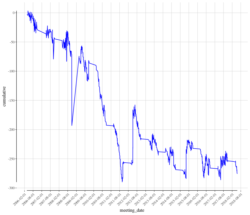
The years 2009 through to the end of 2011 look to be particularly poor years for Aiden O’Brien in Group races, but 2014 onwards has been much more stable.
Today we have shown that just because the trainer may have the best historic strike rate in Group races, backing all of their runners blindly does not necessarily result in a profit. The market obviously knows the A P O’Brien has a very good record in these types of races and his horses are priced accordingly.
An exercise for the reader could be to calculate the P&L for Aiden O’Brien runners when ridden by Ryan Moore. To do this, start by filtering the historic obrien_group_races_only data by R L Moore. Hint: The answer is they are an profitable combination over 375 runs since 2006.
Questions and queries about this article should be posted as a comment below or to the Betwise Q&A board.
The full R code used in this article is found below.
# Load the RMySQL and dplyr library packages
library("RMySQL")
library("dplyr")

# Execute an SQL command to return some historic data
# Connect to the Smartform database. Substitute the placeholder credentials for your own.
# The IP address can be substituted for a remote location if appropriate.
con <- dbConnect(MySQL(),
                        host='127.0.0.1',
                        user='yourusername',
                        password='yourpassword',
                        dbname='smartform')

# This SQL query selects the required columns from the historic_races and historic_runners tables, joining by unique race_id and filtering for results only since January 1st, 2006. The SQL query is saved in a variable called sql1.
sql1 <- paste("SELECT historic_races.course,
              historic_races.meeting_date,
              historic_races.conditions,
              historic_races.group_race,
              historic_races.race_type_id,
              historic_races.race_type,
              historic_runners.name,
              historic_runners.jockey_name,
              historic_runners.trainer_name,
              historic_runners.finish_position,
              historic_runners.starting_price_decimal
              FROM smartform.historic_runners
              JOIN smartform.historic_races USING (race_id)
              WHERE historic_races.meeting_date >= '2006-01-01'", sep="")

# Now execute the SQL query, using the previously established connection. Results are stored in a variable called smartform_results.
smartform_results <- dbGetQuery(con, sql1)

# Close the database connection, which is good practice
dbDisconnect(con)

# Race type IDs 12 and 15 correspond to Flat and All Weather races
flat_races_only <- dplyr::filter(smartform_results,
                                  race_type_id == 12 |
                                   race_type_id == 15)

# Filter using the group_race field for Group 1, 2 and 3 races only
group_races_only <- dplyr::filter(flat_races_only,
                                group_race == 1 |
                                  group_race == 2 |
                                  group_race == 3 )

# For each trainer name, count the number of runs
trainer_group_runs % count(trainer_name)

# Rename the second column in trainer_group_rides to something more logical
names(trainer_group_runs)[2]<-"group_runs"

# Now filter for only winning runs
group_winners_only <- dplyr::filter(group_races_only,
                                    finish_position == 1)

# For each trainer, count the number of winning runs
trainer_group_wins % count(trainer_name)

# Rename the second column in trainer_group_wins to something more logical
names(trainer_group_wins)[2]<-"group_wins"

# Join the two dataframes, trainer_group_runs and trainer_group_wins together, using trainer_name as a key
trainer_group_data <- dplyr::full_join(trainer_group_runs, trainer_group_wins, by = "trainer_name")


# Rename all the NA fields in the new dataframe to zero
# If a trainer has not had a group winner, the group_wins field will be NA
# If this is not changed to zero, later calculations will fail
trainer_group_data[is.na(trainer_group_data)] <- 0

# Now calculate the Group race strike rate for all trainers
trainer_group_data$strike_rate <- (trainer_group_data$group_wins / trainer_group_data$group_runs) * 100

# Execute an SQL command to return some daily data
# Connect to the Smartform database. Substitute the placeholder credentials for your own.
# The IP address can be substituted for a remote location if appropriate.
con <- dbConnect(MySQL(),
                        host='127.0.0.1',
                        user='yourusername',
                        password='yourpassword',
                        dbname='smartform')

# This SQL query selects the required columns from the daily_races and daily_runners tables, joining by unique race_id and filtering for results only with today's date. The SQL query is saved in a variable called sql2.
sql2 <- paste("SELECT daily_races.course,
              daily_races.race_title,
              daily_races.meeting_date,
              daily_runners.name,
              daily_runners.jockey_name,
              daily_runners.trainer_name
              FROM smartform.daily_races
              JOIN smartform.daily_runners USING (race_id)
              WHERE daily_races.meeting_date >='2018-05-18'", sep="")

# Now execute the SQL query, using the previously established connection. Results are stored in a variable called smartform_daily_results.
smartform_daily_results <- dbGetQuery(con, sql2)

# Close the database connection, which is good practice
dbDisconnect(con)

# Filter for the Lockinge Stakes only
lockinge_only <- dplyr::filter(smartform_daily_results,
                              grepl("Lockinge", race_title))

# Using dplyr, join the lockinge_only and trainer_group_data dataframes
lockinge_only_with_sr <- dplyr::inner_join(lockinge_only, trainer_group_data, by = "trainer_name")

# Filter historic data just for A P O'Brien horses
obrien_group_races_only <- dplyr::filter(group_races_only,
                                         grepl("A P O'Brien", trainer_name))

# Non Runners appears as NA, which need to be removed for a true picture and so calulations do not fail
obrien_group_races_only <- dplyr::filter(obrien_group_races_only, !is.na(finish_position))

# Calculate the cumulative total for all O'Brien runners
obrien_cumulative <- cumsum(
  ifelse(obrien_group_races_only$finish_position == 1, (obrien_group_races_only$starting_price_decimal-1),-1)
)

# Add a new column back into obrien_group_races_only, with the cumulative totals
obrien_group_races_only$cumulative <- obrien_cumulative

# Load relevant libraries
library("ggplot2")
library("ggthemes")
library("scales")

# Convert the meeting_date column from character format to Date format
obrien_group_races_only$meeting_date <- as.Date(obrien_group_races_only$meeting_date)

# Plot the chart
ggplot(data=obrien_group_races_only, aes(x=meeting_date, y=cumulative, group=1)) +
  geom_line(colour="blue", lwd=0.7) +
  scale_x_date(labels = date_format("%Y-%m-%d"), date_breaks="6 months") +
  scale_y_continuous(breaks = seq(-300, 10, by = 50)) +
  theme_tufte(base_family="serif", base_size = 14) +
  geom_rangeframe() +
  theme(axis.text.x = element_text(angle = 45, hjust = 1),
        panel.grid.major.x = element_line(color = "grey80"),
        panel.grid.major.y = element_line(color = "grey80"))

##################################################################################
# Reader Exercise: Aiden O'Brien and Ryan Moore combined in Group Races
##################################################################################

obrien_moore_group_races_only <- dplyr::filter(obrien_group_races_only,
                                               grepl("R L Moore", jockey_name))

obrien_moore_cumulative <- cumsum(
  ifelse(obrien_moore_group_races_only$finish_position == 1, (obrien_moore_group_races_only$starting_price_decimal-1),-1)
)

obrien_moore_group_races_only$cumulative <- obrien_moore_cumulative


obrien_moore_group_races_only$meeting_date <- as.Date(obrien_moore_group_races_only$meeting_date)


ggplot(data=obrien_moore_group_races_only, aes(x=meeting_date, y=cumulative, group=1)) +
  geom_line(colour="blue", lwd=0.7) +
  scale_x_date(labels = date_format("%Y-%m-%d"), date_breaks="6 months") +
  theme_tufte(base_family="serif", base_size = 14) +
  geom_rangeframe() +
  theme(axis.text.x = element_text(angle = 45, hjust = 1),
        panel.grid.major.x = element_line(color = "grey80"),
        panel.grid.major.y = element_line(color = "grey80"))
Daily trainer strike rates – how to match for all today’s runners
Saturday, May 12th, 2018Today we’re going to build on the last SQL post where we created a query for 14 day strike rates for all trainers who had runners in the past 14 days. It’s all very well knowing how trainers have performed in the last 14 days, but in practice the way we’ll typically want to use that information is to match the strike rates with today’s runners, so we can compare trainer strike rates within a race.
That is what today’s query is going to show. We’ll be converting the query from the last blog post to a new database table, then querying that table with a left outer join combined with data on today’s runners. First, here’s the query that you can run in Smartform yourself, then we’ll explain what is going on.
-- If the temp table exists delete it

DROP TABLE IF EXISTS temp_trainer_stats_table;

-- create the temporary table by using the first query
CREATE TABLE temp_trainer_stats_table AS (
Select a.*,
ROUND(Winners/Runners * 100,0) AS WinPct,
ROUND(Placers/Runners * 100,0) AS PlacePct
from(
SELECT hru.trainer_name as Trainer, hru.trainer_id,
COUNT(*) AS Runners,
SUM(CASE WHEN hru.finish_position = 1 THEN 1 ELSE 0 END) AS Winners,
sum(case when hra.num_runners < 8 then case when hru.finish_position in ( 2) then 1 else 0 end
else
case when hra.num_runners < 16 then case when hru.finish_position in ( 2,3) then 1 else 0 end
else
case when hra.handicap = 1 then case when hru.finish_position in (2,3,4) then 1 else 0 end
else
case when hru.finish_position in ( 1,2,3) then 1 else 0 end
end
end
end )as Placers,
ROUND(((SUM(CASE WHEN hru.finish_position = 1 THEN (hru.starting_price_decimal -1) ELSE -1 END))),2) AS WinProfit
FROM historic_runners hru
JOIN historic_races hra USING (race_id)
WHERE hra.meeting_date >= ADDDATE(CURDATE(), INTERVAL -14 DAY)
and hra.race_type_id in( 15, 12)
and hru.in_race_comment <> 'Withdrawn'
and hru.starting_price_decimal IS NOT NULL
GROUP BY trainer_name, trainer_id) a);

-- Join the daily runners and daily races to get details of todays card, then do a LEFT OUTER JOIN to get the trainer stats,
-- Where no trainer stats exist NULLS are shown

SELECT substr(dra.scheduled_time, 12,5) as Time, dra.course as Course,
dru.cloth_number as 'No.', dru.name as Horse,
case when dru.stall_number is NULL then "" ELSE dru.stall_number end as Draw, dru.jockey_name as Jockey,
dru.forecast_price as FSP, tmp.*
from daily_races dra
join daily_runners dru using (race_id)
LEFT OUTER JOIN temp_trainer_stats_table tmp using (trainer_id )
where dra.race_type = 'Flat'
and dra.meeting_date = adddate(curdate(), INTERVAL 0 DAY)
-- add a condition here if you want to restrict stats for trainers with less than a certain number of runners
-- eg. [ and runners >=5 ]
order by Time, dru.cloth_number;
Having created a temporary table with the trainer statistics, we now want to join this data to the race card.
The race card data is held in two tables – daily_races and daily runners – which we will join together using the race_id
from daily_races dra
join daily_runners dru using (race_id)
To this we also want to the join the temp_trainer_stats_table we have just created – for this we use a LEFT OUTER JOIN.
This type of join ensures we have the data for every runner in every race on the card, and the trainer data for trainers for which it exists.
For each table I use an identifier eg. Dra for daily_races, tmp for the temp_trainer_stats_table, this enables correct identification of data fields which exist in more than one table.
There is far more data available in the race card data that I am using here, but the basics are:
Time – for this I am using a substring function of the scheduled_time data element, the whole value is for example 2018-05-06 13:30:00 using substr(dra.scheduled_time, 12,5). I am using 5 characters from position 12 which gives me 13:30.
We could also use this to extract the date. There is also a meeting_data data element. Using either of them you can create a date field using a substring and concatenation function like this:
concat(substr(dra.scheduled_time, 9,2),'-',substr(dra.scheduled_time, 6,2),'-',substr(dra.scheduled_time, 1,4)) as RaceDate
Added to the join of the race card data and the trainer data are two conditions to get only flat races for today
where dra.race_type  = 'Flat'
and dra.meeting_date = adddate(curdate(), INTERVAL 0 DAY)
Further criteria could be added to limit the selection to trainers with more than a certain number of runners (eg greater than 4) in the 14 day analysed period
and tmp.runners > 4
and with a strike race greater or equal to 20%
and WinPct >=20
combinations of win percentage, win profit and number of runners would look like this
where dra.race_type  = 'Flat'
and dra.meeting_date = adddate(curdate(), INTERVAL 0 DAY)
and tmp.runners > 4
and tmp.WinPct >= 20
and tmp.WinProfit > 0
Running the first query gives us a result set of 488 rows, neatly ordered by rate time for each of today’s races. We’ve attached a CSV of the output for all today’s races, so you can analyse each race according to trainer strike rate and profitability – something you can of course do for yourself every day in Smartform.
CSV Download: 14 day trainer strike rates for every race on Saturday 12th May
In the next post, we’ll look at different options for automating this query on a daily basis.
Jockey SR% in Group Races and Today’s 1000 Guineas
Sunday, May 6th, 2018Last week we looked at a very simple use of Smartform and R to calculate a single jockey’s strike rate. While a decent introduction, the outcome was not particularly useful. Today we’ll extend this example, in a topical manner, to calculate the Group race strike rate of every jockey riding in the 1000 Guineas at Newmarket.
To begin, load the relevant R libraries and execute an SQL query to return some historic data:
# Load the RMySQL and dplyr library packages
library("RMySQL")
library("dplyr")

# Execute an SQL command to return some historic data
# Connect to the Smartform database. Substitute the placeholder credentials for your own.
# The IP address can be substituted for a remote location if appropriate.
con <- dbConnect(MySQL(),
                        host='127.0.0.1',
                        user='yourusername',
                        password='yourpassword',
                        dbname='smartform')

# This SQL query selects the required columns from the historic_races and historic_runners tables, joining by unique race_id and filtering for results only since January 1st, 2006. The SQL query is saved in a variable called sql1.
sql1 <- paste("SELECT historic_races.course,
              historic_races.conditions,
              historic_races.group_race,
              historic_races.race_type_id,
              historic_races.race_type,
              historic_runners.name,
              historic_runners.jockey_name,
              historic_runners.finish_position
              FROM smartform.historic_runners
              JOIN smartform.historic_races USING (race_id)
              WHERE historic_races.meeting_date >= '2006-01-01'", sep="")

# Now execute the SQL query, using the previously established connection. Results are stored in a variable called smartform_results.
smartform_results <- dbGetQuery(con, sql1)

# Close the database connection, which is good practice
dbDisconnect(con)
The variable smartform_results now contains a large selection of historic data, which can be used to filter and calculate jockey strike rates. In R there are always multiple methods to achieve the same result. The example code used in this article tries to keep things simple, laying out the steps in a logical manner. There are cleaner, faster and perhaps better ways to achieve the goal, some of which will be explored in future posts.
Next, filter for just flat Group races. The vertical bar, |, in the code below corresponds to an OR statement in SQL:
# Race type IDs 12 and 15 correspond to Flat and All Weather races
flat_races_only <- dplyr::filter(smartform_results,
                                  race_type_id == 12 |
                                   race_type_id == 15)

# Filter using the group_race field for Group 1, 2 and 3 races only
group_races_only <- dplyr::filter(flat_races_only,
                                group_race == 1 |
                                  group_race == 2 |
                                  group_race == 3 )
The variable group_races_only now contains details of every Flat and All Weather Group race in the Smartform database since January 1st, 2006.
Using this data, the next step is to calculate strike rates of every jockey who has ever ridden in a Group race. The strange looking symbol linking variables in the code below is a pipe command from the dplyr library:
# For each jockey name, count the number of rides
jockey_group_rides <- group_races_only %>% count(jockey_name)

# Rename the second column in jockey_group_rides to something more logical
names(jockey_group_rides)[2]<-"group_rides"

# Now filter for only winning rides
group_winners_only <- dplyr::filter(group_races_only,
                              finish_position == 1)

# For each jockey, count the number of winning rides
jockey_group_wins <- group_winners_only %>% count(jockey_name)

# Rename the second column in jockey_group_wins to something more logical
names(jockey_group_wins)[2]<-"group_wins"

# Join the two dataframes, jockey_group_rides and jockey_group_wins together, using jockey_name as a key
jockey_group_data <- dplyr::full_join(jockey_group_rides, jockey_group_wins, by = "jockey_name")

# Rename all the NA fields in the new dataframe to zero
# If a jockey has not ridden a group winner, the group_wins field will be NA
# If this is not changed to zero, later calculations will fail
jockey_group_data[is.na(jockey_group_data)] <- 0

# Now calculate the Group race strike rate for all jockeys
jockey_group_data$strike_rate <- (jockey_group_data$group_wins / jockey_group_data$group_rides) * 100
The variable jockey_group_data now contains the strike rate for every jockey who has ridden in a flat or all weather Group race since January 1st, 2006.
While this may be interesting data, it is perhaps not particularly useful on its own. There are some jockeys with a 100% strike rate, from just one ride.
Next step is to apply this data to today’s 1000 Guineas at Newmarket. To begin, another SQL query is required to return daily racing data.
# Execute an SQL command to return some historic data
# Connect to the Smartform database. Substitute the placeholder credentials for your own.
# The IP address can be substituted for a remote location if appropriate.
con <- dbConnect(MySQL(),
                        host='127.0.0.1',
                        user='yourusername',
                        password='yourpassword',
                        dbname='smartform')

# This SQL query selects the required columns from the daily_races and daily_runners tables, joining by unique race_id and filtering for results only with today's date. The SQL query is saved in a variable called sql2.
sql2 <- paste("SELECT daily_races.course,
              daily_races.race_title,
              daily_races.meeting_date,
              daily_runners.name,
              daily_runners.jockey_name
              FROM smartform.daily_races
              JOIN smartform.daily_runners USING (race_id)
              WHERE daily_races.meeting_date >='2018-05-06'", sep="")

# Now execute the SQL query, using the previously established connection. Results are stored in a variable called smartform_daily_results.
smartform_daily_results <- dbGetQuery(con, sql2)

# Close the database connection, which is good practice
dbDisconnect(con)
The variable smartform_daily_results contains information about all races being run today.
The next step is to filter just for the 1000 Guineas. To do this, a grep command is used, which conducts a string match on the race_title field.
# Filter for the 1000 Guineas only
guineas_only <- dplyr::filter(smartform_daily_results,
                              grepl("1000 Guineas", race_title))
The variable guineas_only now contains just the basic details for today’s 1000 Guineas.
Lastly, dplyr is again used to perform a different type of join, which combines the guineas_only and jockey_group_data dataframes, using jockey_name as the key.
# Using dplyr, join the guineas_only and jockey_group_data dataframes
guineas_only_with_sr <- dplyr::inner_join(guineas_only, jockey_group_data, by = "jockey_name")
This results in a new dataframe, guineas_only_with_sr, which contains three new columns, group_rides, group_wins and strike_rate.
It should be no surprise that Ryan Moore has the highest strike rate, from a very large sample size of rides, followed by Frankie Dettori, also with a solid number of rides. Jockeys such as Jim Crowley and Silvestre De Sousa should be carefully considered, as they both have a significant sample size of rides, but quite a low winning strike rate.
> guineas_only_with_sr

      course                                   race_title meeting_date            name   jockey_name group_rides group_wins strike_rate
1  Newmarket Qipco 1000 Guineas Stakes (Fillies' Group 1)   2018-05-06      Altyn Orda     L Dettori         980        160   16.326531
2  Newmarket Qipco 1000 Guineas Stakes (Fillies' Group 1)   2018-05-06     Anna Nerium  Tom Marquand          18          1    5.555556
3  Newmarket Qipco 1000 Guineas Stakes (Fillies' Group 1)   2018-05-06 Billesdon Brook     S M Levey         130          5    3.846154
4  Newmarket Qipco 1000 Guineas Stakes (Fillies' Group 1)   2018-05-06     Dan's Dream    S De Sousa         316         23    7.278481
5  Newmarket Qipco 1000 Guineas Stakes (Fillies' Group 1)   2018-05-06         Happily     R L Moore        1281        250   19.516003
6  Newmarket Qipco 1000 Guineas Stakes (Fillies' Group 1)   2018-05-06       I Can Fly J A Heffernan         571         62   10.858144
7  Newmarket Qipco 1000 Guineas Stakes (Fillies' Group 1)   2018-05-06         Laurens    P McDonald          37          5   13.513514
8  Newmarket Qipco 1000 Guineas Stakes (Fillies' Group 1)   2018-05-06    Liquid Amber       W J Lee         164         13    7.926829
9  Newmarket Qipco 1000 Guineas Stakes (Fillies' Group 1)   2018-05-06        Madeline Andrea Atzeni         357         52   14.565826
10 Newmarket Qipco 1000 Guineas Stakes (Fillies' Group 1)   2018-05-06       Sarrocchi    W M Lordan         357         42   11.764706
11 Newmarket Qipco 1000 Guineas Stakes (Fillies' Group 1)   2018-05-06        Sizzling     D O'Brien          98         10   10.204082
12 Newmarket Qipco 1000 Guineas Stakes (Fillies' Group 1)   2018-05-06       Soliloquy       W Buick         338         44   13.017751
13 Newmarket Qipco 1000 Guineas Stakes (Fillies' Group 1)   2018-05-06         Vitamin   Jim Crowley         471         39    8.280255
14 Newmarket Qipco 1000 Guineas Stakes (Fillies' Group 1)   2018-05-06   Wild Illusion   James Doyle         372         46   12.365591
15 Newmarket Qipco 1000 Guineas Stakes (Fillies' Group 1)   2018-05-06         Worship  Oisin Murphy         195         16    8.205128
Looking at such a table is interesting, but not very visually appealing. Some people also understand data better when it is presented in chart form, rather than simple numbers in a table. Therefore, we’ll now briefly look at plotting jockey’s Group strike rates as a bar chart.
To do this, another popular R library called ggplot will be used. The code below creates a simple bar chart:
# Load the ggplot library
library(ggplot2)

# Create a new variable with the jockey name and strike rate data as x and y axis
sr_bar <- ggplot(guineas_only_with_sr, aes(jockey_name, strike_rate))

# Using the sr_bar variable, create a column chart, with blue bars and the x axis labels at a 90% angle from horizontal
sr_bar + geom_col(colour = "blue", fill = "blue") +
  theme(axis.text.x = element_text(angle = 90, hjust = 1))
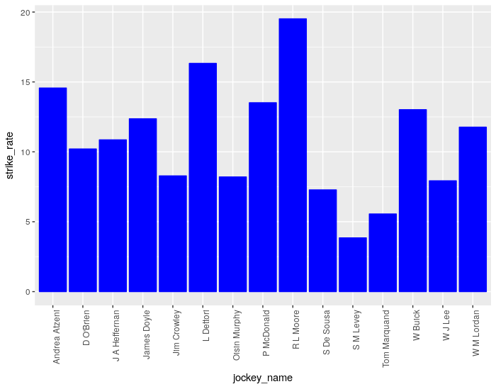
This chart makes it obvious that Moore and Dettori have the two superior strike rates when riding in Group races.
Ggplot is a very powerful charting library, with huge number of options. An Rstudio cheatsheet helps to explain some of the most common options.
Further information regarding using the dplyr library, which has a wide range of very useful data manipulation functions, can be found in this RStudio cheatsheet.
This tutorial could be easily extended to produce trainer or even sire strike rates in Group races, which could provide further useful insights into today’s 1000 Guineas.
Questions and queries about this article should be posted as a comment below or to the Betwise Q&A board.
The full R code used in this article is found below.
# Load the RMySQL and dplyr library packages
library("RMySQL")
library("dplyr")

# Execute an SQL command to return some historic data
# Connect to the Smartform database. Substitute the placeholder credentials for your own.
# The IP address can be substituted for a remote location if appropriate.
con <- dbConnect(MySQL(),
                        host='127.0.0.1',
                        user='yourusername',
                        password='yourpassword',
                        dbname='smartform')

# This SQL query selects the required columns from the historic_races and historic_runners tables, joining by unique race_id and filtering for results only since January 1st, 2006. The SQL query is saved in a variable called sql1.
sql1 <- paste("SELECT historic_races.course,
              historic_races.conditions,
              historic_races.group_race,
              historic_races.race_type_id,
              historic_races.race_type,
              historic_runners.name,
              historic_runners.jockey_name,
              historic_runners.finish_position
              FROM smartform.historic_runners
              JOIN smartform.historic_races USING (race_id)
              WHERE historic_races.meeting_date >= '2006-01-01'", sep="")

# Now execute the SQL query, using the previously established connection. Results are stored in a variable called smartform_results.
smartform_results <- dbGetQuery(con, sql1)

# Close the database connection, which is good practice
dbDisconnect(con)

# Race type IDs 12 and 15 correspond to Flat and All Weather races
flat_races_only <- dplyr::filter(smartform_results,
                                  race_type_id == 12 |
                                   race_type_id == 15)

# Filter using the group_race field for Group 1, 2 and 3 races only
group_races_only <- dplyr::filter(flat_races_only,
                                group_race == 1 |
                                  group_race == 2 |
                                  group_race == 3 )

# For each jockey name, count the number of rides
jockey_group_rides <- group_races_only %>% count(jockey_name)

# Rename the second column in jockey_group_rides to something more logical
names(jockey_group_rides)[2]<-"group_rides"

# Now filter for only winning rides
group_winners_only <- dplyr::filter(group_races_only,
                              finish_position == 1)

# For each jockey, count the number of winning rides
jockey_group_wins <- group_winners_only %>% count(jockey_name)

# Rename the second column in jockey_group_wins to something more logical
names(jockey_group_wins)[2]<-"group_wins"

# Join the two dataframes, jockey_group_rides and jockey_group_wins together, using jockey_name as a key
jockey_group_data <- dplyr::full_join(jockey_group_rides, jockey_group_wins, by = "jockey_name")

# Rename all the NA fields in the new dataframe to zero
# If a jockey has not ridden a group winner, the group_wins field will be NA
# If this is not changed to zero, later calculations will fail
jockey_group_data[is.na(jockey_group_data)] <- 0

# Now calculate the Group race strike rate for all jockeys
jockey_group_data$strike_rate <- (jockey_group_data$group_wins / jockey_group_data$group_rides) * 100

# Execute an SQL command to return some historic data
# Connect to the Smartform database. Substitute the placeholder credentials for your own.
# The IP address can be substituted for a remote location if appropriate.
con <- dbConnect(MySQL(),
                        host='127.0.0.1',
                        user='yourusername',
                        password='yourpassword',
                        dbname='smartform')

# This SQL query selects the required columns from the daily_races and daily_runners tables, joining by unique race_id and filtering for results only with today's date. The SQL query is saved in a variable called sql2.
sql2 <- paste("SELECT daily_races.course,
              daily_races.race_title,
              daily_races.meeting_date,
              daily_runners.name,
              daily_runners.jockey_name
              FROM smartform.daily_races
              JOIN smartform.daily_runners USING (race_id)
              WHERE daily_races.meeting_date >='2018-05-06'", sep="")

# Now execute the SQL query, using the previously established connection. Results are stored in a variable called smartform_daily_results.
smartform_daily_results <- dbGetQuery(con, sql2)

# Close the database connection, which is good practice
dbDisconnect(con)

# Filter for the 1000 Guineas only
guineas_only <- dplyr::filter(smartform_daily_results,
                              grepl("1000 Guineas", race_title))

# Using dplyr, join the guineas_only and jockey_group_data dataframes
guineas_only_with_sr <- dplyr::inner_join(guineas_only, jockey_group_data, by = "jockey_name")

# Load the ggplot library
library(ggplot2)

# Create a new variable with the jockey name and strike rate data as x and y axis
sr_bar <- ggplot(guineas_only_with_sr, aes(jockey_name, strike_rate))

# Using the sr_bar variable, create a column chart, with blue bars and the x axis labels at a 90% angle from horizontal
sr_bar + geom_col(colour = "blue", fill = "blue") +
  theme(axis.text.x = element_text(angle = 90, hjust = 1))
Daily trainer strike rates in Smartform
Saturday, May 5th, 2018There are many ways to skin a cat in Smartform. One of the simplest is to stick with SQL and stay in the database, without resorting to programming or exporting the data.
So here is a breakdown of how to generate one of the most commonly used “derived” statistics in horseracing – trainer strike rates. We hear that trainers whose horses are currently in good form are worth backing – but how can we tell?
The following single SQL produces Trainer strike rates for all daily Flat races in the database, calculated over a period of 14 days. Copy and paste the code at your MySQL command prompt:
Select a.*,

ROUND(Winners/Runners * 100,0) AS WinPct,
ROUND(Placers/Runners * 100,0) AS PlacePct

from(

SELECT hru.trainer_name as Trainer, hru.trainer_id,

COUNT(*) AS Runners,

SUM(CASE WHEN hru.finish_position = 1 THEN 1 ELSE 0 END) AS Winners,

sum(case when hra.num_runners < 8 then case when hru.finish_position in ( 2)  then 1 else 0 end

else

case when hra.num_runners < 16 then case when hru.finish_position in ( 2,3)  then 1 else 0 end

else

case when hra.handicap = 1 then case when hru.finish_position in (2,3,4) then 1 else 0 end

else

case when hru.finish_position in ( 1,2,3)  then 1 else 0 end

end

end

end )as Placers,

ROUND(((SUM(CASE WHEN hru.finish_position = 1 THEN (hru.starting_price_decimal -1) ELSE -1 END))),2) AS WinProfit

FROM historic_runners hru

JOIN historic_races hra USING (race_id)

WHERE hra.meeting_date >= ADDDATE(CURDATE(), INTERVAL -14 DAY)

and hra.race_type_id  in( 15, 12)
and hru.in_race_comment <> 'Withdrawn'
and hru.starting_price_decimal IS NOT NULL

GROUP BY trainer_name, trainer_id

) a

Where runners >= 5 or winners >= 3

ORDER BY  WinProfit desc
LIMIT 20;
The approach is to generate a query within a query – to allow the use of the counts done in the main query to be used to create the strike rate percentages.
The main part joins the historic_runners and historic_races tables by race_id.
The WHERE clause defines the criteria
Firstly, define the period over which you want the analysis, here we set it to analyze races in the last 14 days
hra.meeting_date >= ADDDATE(CURDATE(), INTERVAL -14 DAY)
Secondly we define the race types for all Flat races (12 for Turf and 15 for All Weather)
All of these can be found running the SQL statement:
select distinct race_type, race_type_id from historic_races; )
The final criteria helps to eliminate horses who have not actually participated that are in the database, non-runners, withdrawn etc. There are a number of ways to do this and one can find their own criteria, but I use this:
and hru.in_race_comment <> 'Withdrawn'
and hru.starting_price_decimal IS NOT NULL
The outer section of the SQL selects all the data from the inner part and displays it and calculates the strike rates. The )a afterwards is required by SQL.
Finally in Green are the sorting instructions and some other criteria.
Also note that here I am choosing to only display trainers who have had at least 5 runners or at least 3 winners.
Where runners >= 5

or winners >= 3
I am ordering them in order of greatest win profit
ORDER BY WinProfit desc
And limiting the number of trainers displayed to 20
LIMIT 20
So on the day of the 2000 Guineas, Brian Meehan is currently the most profitable trainer to follow, with £47 retuns, but P W Hiatt has the highest strike rate, with 60% – albeit with only 5 runners in the last few days.
If you’re looking for a trainer with a high strike rate from at leasy double digit runners in the last 14 days, then Mark Usher, with a 33% win strike and 25% place strike, is impressive.
Adapt the SQL above to generate daily trainer strike rates so you can judge for yourself.