
Jockey SR% in Group Races and Today’s 1000 Guineas
By Phill Clarke on Sunday, May 6th, 2018Last week we looked at a very simple use of Smartform and R to calculate a single jockey’s strike rate. While a decent introduction, the outcome was not particularly useful. Today we’ll extend this example, in a topical manner, to calculate the Group race strike rate of every jockey riding in the 1000 Guineas at Newmarket.
To begin, load the relevant R libraries and execute an SQL query to return some historic data:
# Load the RMySQL and dplyr library packages
library("RMySQL")
library("dplyr")

# Execute an SQL command to return some historic data
# Connect to the Smartform database. Substitute the placeholder credentials for your own.
# The IP address can be substituted for a remote location if appropriate.
con <- dbConnect(MySQL(),
                        host='127.0.0.1',
                        user='yourusername',
                        password='yourpassword',
                        dbname='smartform')

# This SQL query selects the required columns from the historic_races and historic_runners tables, joining by unique race_id and filtering for results only since January 1st, 2006. The SQL query is saved in a variable called sql1.
sql1 <- paste("SELECT historic_races.course,
              historic_races.conditions,
              historic_races.group_race,
              historic_races.race_type_id,
              historic_races.race_type,
              historic_runners.name,
              historic_runners.jockey_name,
              historic_runners.finish_position
              FROM smartform.historic_runners
              JOIN smartform.historic_races USING (race_id)
              WHERE historic_races.meeting_date >= '2006-01-01'", sep="")

# Now execute the SQL query, using the previously established connection. Results are stored in a variable called smartform_results.
smartform_results <- dbGetQuery(con, sql1)

# Close the database connection, which is good practice
dbDisconnect(con)
The variable smartform_results now contains a large selection of historic data, which can be used to filter and calculate jockey strike rates. In R there are always multiple methods to achieve the same result. The example code used in this article tries to keep things simple, laying out the steps in a logical manner. There are cleaner, faster and perhaps better ways to achieve the goal, some of which will be explored in future posts.
Next, filter for just flat Group races. The vertical bar, |, in the code below corresponds to an OR statement in SQL:
# Race type IDs 12 and 15 correspond to Flat and All Weather races
flat_races_only <- dplyr::filter(smartform_results,
                                  race_type_id == 12 |
                                   race_type_id == 15)

# Filter using the group_race field for Group 1, 2 and 3 races only
group_races_only <- dplyr::filter(flat_races_only,
                                group_race == 1 |
                                  group_race == 2 |
                                  group_race == 3 )
The variable group_races_only now contains details of every Flat and All Weather Group race in the Smartform database since January 1st, 2006.
Using this data, the next step is to calculate strike rates of every jockey who has ever ridden in a Group race. The strange looking symbol linking variables in the code below is a pipe command from the dplyr library:
# For each jockey name, count the number of rides
jockey_group_rides <- group_races_only %>% count(jockey_name)

# Rename the second column in jockey_group_rides to something more logical
names(jockey_group_rides)[2]<-"group_rides"

# Now filter for only winning rides
group_winners_only <- dplyr::filter(group_races_only,
                              finish_position == 1)

# For each jockey, count the number of winning rides
jockey_group_wins <- group_winners_only %>% count(jockey_name)

# Rename the second column in jockey_group_wins to something more logical
names(jockey_group_wins)[2]<-"group_wins"

# Join the two dataframes, jockey_group_rides and jockey_group_wins together, using jockey_name as a key
jockey_group_data <- dplyr::full_join(jockey_group_rides, jockey_group_wins, by = "jockey_name")

# Rename all the NA fields in the new dataframe to zero
# If a jockey has not ridden a group winner, the group_wins field will be NA
# If this is not changed to zero, later calculations will fail
jockey_group_data[is.na(jockey_group_data)] <- 0

# Now calculate the Group race strike rate for all jockeys
jockey_group_data$strike_rate <- (jockey_group_data$group_wins / jockey_group_data$group_rides) * 100
The variable jockey_group_data now contains the strike rate for every jockey who has ridden in a flat or all weather Group race since January 1st, 2006.
While this may be interesting data, it is perhaps not particularly useful on its own. There are some jockeys with a 100% strike rate, from just one ride.
Next step is to apply this data to today’s 1000 Guineas at Newmarket. To begin, another SQL query is required to return daily racing data.
# Execute an SQL command to return some historic data
# Connect to the Smartform database. Substitute the placeholder credentials for your own.
# The IP address can be substituted for a remote location if appropriate.
con <- dbConnect(MySQL(),
                        host='127.0.0.1',
                        user='yourusername',
                        password='yourpassword',
                        dbname='smartform')

# This SQL query selects the required columns from the daily_races and daily_runners tables, joining by unique race_id and filtering for results only with today's date. The SQL query is saved in a variable called sql2.
sql2 <- paste("SELECT daily_races.course,
              daily_races.race_title,
              daily_races.meeting_date,
              daily_runners.name,
              daily_runners.jockey_name
              FROM smartform.daily_races
              JOIN smartform.daily_runners USING (race_id)
              WHERE daily_races.meeting_date >='2018-05-06'", sep="")

# Now execute the SQL query, using the previously established connection. Results are stored in a variable called smartform_daily_results.
smartform_daily_results <- dbGetQuery(con, sql2)

# Close the database connection, which is good practice
dbDisconnect(con)
The variable smartform_daily_results contains information about all races being run today.
The next step is to filter just for the 1000 Guineas. To do this, a grep command is used, which conducts a string match on the race_title field.
# Filter for the 1000 Guineas only
guineas_only <- dplyr::filter(smartform_daily_results,
                              grepl("1000 Guineas", race_title))
The variable guineas_only now contains just the basic details for today’s 1000 Guineas.
Lastly, dplyr is again used to perform a different type of join, which combines the guineas_only and jockey_group_data dataframes, using jockey_name as the key.
# Using dplyr, join the guineas_only and jockey_group_data dataframes
guineas_only_with_sr <- dplyr::inner_join(guineas_only, jockey_group_data, by = "jockey_name")
This results in a new dataframe, guineas_only_with_sr, which contains three new columns, group_rides, group_wins and strike_rate.
It should be no surprise that Ryan Moore has the highest strike rate, from a very large sample size of rides, followed by Frankie Dettori, also with a solid number of rides. Jockeys such as Jim Crowley and Silvestre De Sousa should be carefully considered, as they both have a significant sample size of rides, but quite a low winning strike rate.
> guineas_only_with_sr

      course                                   race_title meeting_date            name   jockey_name group_rides group_wins strike_rate
1  Newmarket Qipco 1000 Guineas Stakes (Fillies' Group 1)   2018-05-06      Altyn Orda     L Dettori         980        160   16.326531
2  Newmarket Qipco 1000 Guineas Stakes (Fillies' Group 1)   2018-05-06     Anna Nerium  Tom Marquand          18          1    5.555556
3  Newmarket Qipco 1000 Guineas Stakes (Fillies' Group 1)   2018-05-06 Billesdon Brook     S M Levey         130          5    3.846154
4  Newmarket Qipco 1000 Guineas Stakes (Fillies' Group 1)   2018-05-06     Dan's Dream    S De Sousa         316         23    7.278481
5  Newmarket Qipco 1000 Guineas Stakes (Fillies' Group 1)   2018-05-06         Happily     R L Moore        1281        250   19.516003
6  Newmarket Qipco 1000 Guineas Stakes (Fillies' Group 1)   2018-05-06       I Can Fly J A Heffernan         571         62   10.858144
7  Newmarket Qipco 1000 Guineas Stakes (Fillies' Group 1)   2018-05-06         Laurens    P McDonald          37          5   13.513514
8  Newmarket Qipco 1000 Guineas Stakes (Fillies' Group 1)   2018-05-06    Liquid Amber       W J Lee         164         13    7.926829
9  Newmarket Qipco 1000 Guineas Stakes (Fillies' Group 1)   2018-05-06        Madeline Andrea Atzeni         357         52   14.565826
10 Newmarket Qipco 1000 Guineas Stakes (Fillies' Group 1)   2018-05-06       Sarrocchi    W M Lordan         357         42   11.764706
11 Newmarket Qipco 1000 Guineas Stakes (Fillies' Group 1)   2018-05-06        Sizzling     D O'Brien          98         10   10.204082
12 Newmarket Qipco 1000 Guineas Stakes (Fillies' Group 1)   2018-05-06       Soliloquy       W Buick         338         44   13.017751
13 Newmarket Qipco 1000 Guineas Stakes (Fillies' Group 1)   2018-05-06         Vitamin   Jim Crowley         471         39    8.280255
14 Newmarket Qipco 1000 Guineas Stakes (Fillies' Group 1)   2018-05-06   Wild Illusion   James Doyle         372         46   12.365591
15 Newmarket Qipco 1000 Guineas Stakes (Fillies' Group 1)   2018-05-06         Worship  Oisin Murphy         195         16    8.205128
Looking at such a table is interesting, but not very visually appealing. Some people also understand data better when it is presented in chart form, rather than simple numbers in a table. Therefore, we’ll now briefly look at plotting jockey’s Group strike rates as a bar chart.
To do this, another popular R library called ggplot will be used. The code below creates a simple bar chart:
# Load the ggplot library
library(ggplot2)

# Create a new variable with the jockey name and strike rate data as x and y axis
sr_bar <- ggplot(guineas_only_with_sr, aes(jockey_name, strike_rate))

# Using the sr_bar variable, create a column chart, with blue bars and the x axis labels at a 90% angle from horizontal
sr_bar + geom_col(colour = "blue", fill = "blue") +
  theme(axis.text.x = element_text(angle = 90, hjust = 1))
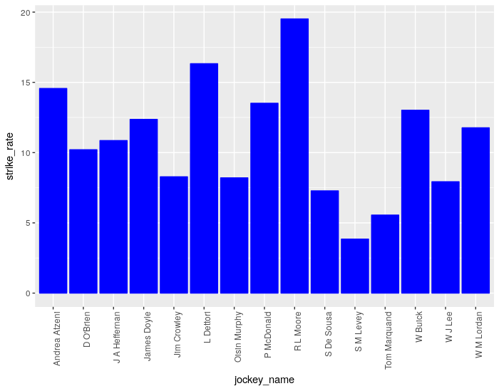
This chart makes it obvious that Moore and Dettori have the two superior strike rates when riding in Group races.
Ggplot is a very powerful charting library, with huge number of options. An Rstudio cheatsheet helps to explain some of the most common options.
Further information regarding using the dplyr library, which has a wide range of very useful data manipulation functions, can be found in this RStudio cheatsheet.
This tutorial could be easily extended to produce trainer or even sire strike rates in Group races, which could provide further useful insights into today’s 1000 Guineas.
Questions and queries about this article should be posted as a comment below or to the Betwise Q&A board.
The full R code used in this article is found below.
# Load the RMySQL and dplyr library packages
library("RMySQL")
library("dplyr")

# Execute an SQL command to return some historic data
# Connect to the Smartform database. Substitute the placeholder credentials for your own.
# The IP address can be substituted for a remote location if appropriate.
con <- dbConnect(MySQL(),
                        host='127.0.0.1',
                        user='yourusername',
                        password='yourpassword',
                        dbname='smartform')

# This SQL query selects the required columns from the historic_races and historic_runners tables, joining by unique race_id and filtering for results only since January 1st, 2006. The SQL query is saved in a variable called sql1.
sql1 <- paste("SELECT historic_races.course,
              historic_races.conditions,
              historic_races.group_race,
              historic_races.race_type_id,
              historic_races.race_type,
              historic_runners.name,
              historic_runners.jockey_name,
              historic_runners.finish_position
              FROM smartform.historic_runners
              JOIN smartform.historic_races USING (race_id)
              WHERE historic_races.meeting_date >= '2006-01-01'", sep="")

# Now execute the SQL query, using the previously established connection. Results are stored in a variable called smartform_results.
smartform_results <- dbGetQuery(con, sql1)

# Close the database connection, which is good practice
dbDisconnect(con)

# Race type IDs 12 and 15 correspond to Flat and All Weather races
flat_races_only <- dplyr::filter(smartform_results,
                                  race_type_id == 12 |
                                   race_type_id == 15)

# Filter using the group_race field for Group 1, 2 and 3 races only
group_races_only <- dplyr::filter(flat_races_only,
                                group_race == 1 |
                                  group_race == 2 |
                                  group_race == 3 )

# For each jockey name, count the number of rides
jockey_group_rides <- group_races_only %>% count(jockey_name)

# Rename the second column in jockey_group_rides to something more logical
names(jockey_group_rides)[2]<-"group_rides"

# Now filter for only winning rides
group_winners_only <- dplyr::filter(group_races_only,
                              finish_position == 1)

# For each jockey, count the number of winning rides
jockey_group_wins <- group_winners_only %>% count(jockey_name)

# Rename the second column in jockey_group_wins to something more logical
names(jockey_group_wins)[2]<-"group_wins"

# Join the two dataframes, jockey_group_rides and jockey_group_wins together, using jockey_name as a key
jockey_group_data <- dplyr::full_join(jockey_group_rides, jockey_group_wins, by = "jockey_name")

# Rename all the NA fields in the new dataframe to zero
# If a jockey has not ridden a group winner, the group_wins field will be NA
# If this is not changed to zero, later calculations will fail
jockey_group_data[is.na(jockey_group_data)] <- 0

# Now calculate the Group race strike rate for all jockeys
jockey_group_data$strike_rate <- (jockey_group_data$group_wins / jockey_group_data$group_rides) * 100

# Execute an SQL command to return some historic data
# Connect to the Smartform database. Substitute the placeholder credentials for your own.
# The IP address can be substituted for a remote location if appropriate.
con <- dbConnect(MySQL(),
                        host='127.0.0.1',
                        user='yourusername',
                        password='yourpassword',
                        dbname='smartform')

# This SQL query selects the required columns from the daily_races and daily_runners tables, joining by unique race_id and filtering for results only with today's date. The SQL query is saved in a variable called sql2.
sql2 <- paste("SELECT daily_races.course,
              daily_races.race_title,
              daily_races.meeting_date,
              daily_runners.name,
              daily_runners.jockey_name
              FROM smartform.daily_races
              JOIN smartform.daily_runners USING (race_id)
              WHERE daily_races.meeting_date >='2018-05-06'", sep="")

# Now execute the SQL query, using the previously established connection. Results are stored in a variable called smartform_daily_results.
smartform_daily_results <- dbGetQuery(con, sql2)

# Close the database connection, which is good practice
dbDisconnect(con)

# Filter for the 1000 Guineas only
guineas_only <- dplyr::filter(smartform_daily_results,
                              grepl("1000 Guineas", race_title))

# Using dplyr, join the guineas_only and jockey_group_data dataframes
guineas_only_with_sr <- dplyr::inner_join(guineas_only, jockey_group_data, by = "jockey_name")

# Load the ggplot library
library(ggplot2)

# Create a new variable with the jockey name and strike rate data as x and y axis
sr_bar <- ggplot(guineas_only_with_sr, aes(jockey_name, strike_rate))

# Using the sr_bar variable, create a column chart, with blue bars and the x axis labels at a 90% angle from horizontal
sr_bar + geom_col(colour = "blue", fill = "blue") +
  theme(axis.text.x = element_text(angle = 90, hjust = 1))