
Posts Tagged ‘Boruta’
Looking at the importance of variables.
Sunday, August 23rd, 2020This article shows how you can compare how important different variables are from the historical insights table in Smartform.
The article provides a skeleton where you can test other variables for other types of races. I have put the whole R code at the end of article
In the Historical Insights table are some new variables. I am going to look at a group of these.
- won_LTO, won_PTO, won_ATO, placed_LTO, placed_PTO, placed_ATO, handicap_LTO. handicap_PTO, handicap_ATO, percent_beaten_LTO, percent_beaten_PTO and percent_beaten_ATO
These are quite self-explanatory with LTO meaning last time out, PTO is penultimate time out and ATO, antepenultimate time out or three runs ago.
I have chosen to look at all UK all-weather handicaps since January 1st 2017. I have chosen handicaps as the runners will generally have several previous runs. I have guaranteed this by only selecting horses that have more than three previous runs.
I will be using a package called Boruta to compare the variables so you will need to install that if you do not already have it.
library("RMySQL")
library("dplyr")
library("reshape2")
library("ggplot2")
library("Boruta")
As always I do a summary of the data. Here I need to deal with NA values, and there are some in the historic_runners.finishing_position field. Because I have over 55000 rows of data and only 250 NAs I have deleted those rows.
smartform_results <- na.omit(smartform_results)I need to add a variable to tell me if the horse has won the race or not, I have called this winner. It will act as a target for my other variables.
smartform_results$Winner = ifelse(smartform_results$finish_position < 2,1,0)Then I need to select the variables I wish to compare in their importance in predicting the winner variable.
allnames=names(smartform_results)
allnames
 [1] "course"                 "meeting_date"           "race_id"                "race_type_id"           "race_type"
 [6] "distance_yards"         "name"                   "finish_position"        "starting_price_decimal" "won_LTO"
[11] "won_PTO"                "won_ATO"                "placed_LTO"             "placed_PTO"             "placed_ATO"
[16] "handicap_LTO"           "handicap_PTO"           "handicap_ATO"           "percent_beaten_LTO"     "percent_beaten_PTO"
[21] "percent_beaten_ATO"     "prev_runs"              "Winner"
This gives me a list of all the variables in my data.
I must admit when downloading data from a database I like to include a variety of race and horse variables to make sure my selection criteria have worked properly. For example race and horse names. I now need to remove these to make a list of the variables I need.
I can see I have 23 variables, and from the output of allnames I can work out which ones I don’t need and get their numerical indices. I find it easier to work with numbers than variable names at this stage. Notice I’ve removed my target variable, winner.
datalist=allnames[-c(1,2,3,4,5,6,7,8,9,22,23)]
> datalist
 [1] "won_LTO"            "won_PTO"            "won_ATO"            "placed_LTO"         "placed_PTO"         "placed_ATO"
 [7] "handicap_LTO"       "handicap_PTO"       "handicap_ATO"       "percent_beaten_LTO" "percent_beaten_PTO" "percent_beaten_ATO"
> target=allnames[23]
> target
[1] "Winner"
So datalist contains all the variables I am testing and target is the target that they are trying to predict.
I use these to produce the formula that R uses for most machine learning and statistical modelling
mlformula <- as.formula(paste(target,paste(datalist,collapse=" + "), sep=" ~ "))All this rather unpleasant looking snippet does is produce this formula.
Winner ~ won_LTO + won_PTO + won_ATO + placed_LTO + placed_PTO +
    placed_ATO + handicap_LTO + handicap_PTO + handicap_ATO +
    percent_beaten_LTO + percent_beaten_PTO + percent_beaten_ATO
This means predict the value of Winner using all the variables after the ~ symbol.
This translates as, predict winner using all the variables named after the ~ symbol.
At last, we can use Boruta to see which of our variables is the most important. I am not going to give a tutorial in using Boruta. There are numerous ones available on the internet. There are various options you can use. I have just run the simple vanilla options here. It will take a little while to run depending on the speed of your machine
Once it has finished, you can do one more thing. This line forces Boruta to decide if variables are important.
final.boruta <- TentativeRoughFix(boruta.train)Here is the output. Do not worry if your numbers do not exactly match they should be similar.
                    meanImp medianImp     minImp    maxImp  normHits  decision
won_LTO            17.454272 17.336936 15.2723929 19.681327 1.0000000 Confirmed
won_PTO            11.858611 11.847156  9.6080635 13.915011 1.0000000 Confirmed
won_ATO            10.646576 10.571548  8.5119054 12.529334 1.0000000 Confirmed
placed_LTO         22.967911 23.035708 20.2490144 25.244789 1.0000000 Confirmed
placed_PTO         21.871156 21.946160 19.2961340 24.466836 1.0000000 Confirmed
placed_ATO         20.242410 20.231261 17.3522156 22.853500 1.0000000 Confirmed
handicap_LTO        2.437791  2.360027 -0.9938698  5.342918 0.4747475 Confirmed
handicap_PTO        7.568926  7.620271  4.2983632 11.147914 1.0000000 Confirmed
handicap_ATO        9.521332  9.551424  5.7088247 13.628699 1.0000000 Confirmed
percent_beaten_LTO 34.039496 34.076843 30.2324486 38.099816 1.0000000 Confirmed
percent_beaten_PTO 27.804420 27.716601 24.2223531 31.686299 1.0000000 Confirmed
percent_beaten_ATO 22.990647 23.121783 19.8763102 25.945583 1.0000000 Confirmed
All the variables are confirmed as being important related to the target variable. The higher the value in the first column the more important the variable. Here the percent beaten variables seem to do well while the handicap last time out is only just significant.
You can see this better in a graph.
plot(boruta.train, xlab = "", xaxt = "n")
lz<-lapply(1:ncol(boruta.train$ImpHistory),function(i) boruta.train$ImpHistory[is.finite(boruta.train$ImpHistory[,i]),i])
names(lz) <- colnames(boruta.train$ImpHistory)
Labels <- sort(sapply(lz,median))
axis(side = 1,las=2,labels = names(Labels), at = 1:ncol(boruta.train$ImpHistory), cex.axis = 0.7)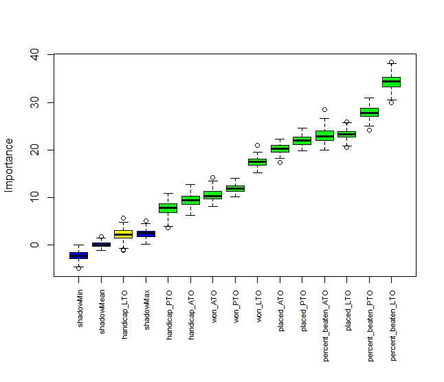
Handicap LTO is yellow as that is only just significant. The rest are green and are significant. The three blue variables are what we might expect by chance, read up more on Boruta for more details..
It is also worth noting for each variable apart from handicap LTO the most recent race is the most significant. SO LTO is more significant than PTO which is more significant than LTO.
By looking at variable importance, we can concentrate our modelling on those that are most important to our outcome
The importance of variables will vary with the type of race you are studying. What is important to all-weather handicaps may well not be important in long-distance Novice Chases.
Hopefully, you can use the attached script as a blueprint for your particular analyses.
library("RMySQL")
library("dplyr")
library("reshape2")
library("ggplot2")
library("Boruta")

con <- dbConnect(MySQL(),
host='127.0.0.1',
user='smartform',
password='*************',
dbname='smartform')
sql1 <- paste("SELECT historic_races.course,
historic_races.meeting_date,
historic_races.race_id,
historic_races.race_type_id,
historic_races.race_type,
historic_races.distance_yards,
historic_runners.name,
historic_runners.finish_position,
historic_runners.starting_price_decimal,
historic_runners_insights.won_LTO,
historic_runners_insights.won_PTO,
historic_runners_insights.won_ATO,
historic_runners_insights.placed_LTO,
historic_runners_insights.placed_PTO,
historic_runners_insights.placed_ATO,
historic_runners_insights.handicap_LTO,
historic_runners_insights.handicap_PTO,
historic_runners_insights.handicap_ATO,
historic_runners_insights.percent_beaten_LTO,
historic_runners_insights.percent_beaten_PTO,
historic_runners_insights.percent_beaten_ATO,
historic_runners_insights.prev_runs
FROM smartform.historic_runners
JOIN smartform.historic_races USING (race_id)
JOIN smartform.historic_runners_insights USING (race_id, runner_id)
WHERE historic_races.meeting_date >= '2019-01-01' AND historic_races.race_type_id=15 AND historic_runners_insights.prev_runs>3 AND historic_races.course!='Dundalk'AND historic_races.handicap=1", sep="")
smartform_results <- dbGetQuery(con, sql1)
View(smartform_results)
dbDisconnect(con)
smartform_results <- na.omit(smartform_results)
smartform_results$Winner = ifelse(smartform_results$finish_position < 2,1,0)
allnames=names(smartform_results)
allnames
datalist=allnames[-c(1,2,3,4,5,6,7,8,9,22,23)]
datalist
target=allnames[23]
target
mlformula <- as.formula(paste(target, paste(datalist,collapse=" + "), sep=" ~ "))
mlformula
print(mlformula)
set.seed(123)
boruta.train <- Boruta(mlformula, data =smartform_results, doTrace = 2)
print(boruta.train)
final.boruta <- TentativeRoughFix(boruta.train)
boruta.df <- attStats(final.boruta)
print(boruta.df)
plot(boruta.train, xlab = "", xaxt = "n")
lz<-lapply(1:ncol(boruta.train$ImpHistory),function(i) boruta.train$ImpHistory[is.finite(boruta.train$ImpHistory[,i]),i])
names(lz) <- colnames(boruta.train$ImpHistory)
Labels <- sort(sapply(lz,median))
axis(side = 1,las=2,labels = names(Labels), at = 1:ncol(boruta.train$ImpHistory), cex.axis = 0.7)