
O’Brien and Moore in Group Races – Scatterplots with R
By Phill Clarke on Saturday, May 26th, 2018Last week we looked at the performance of Aiden O’Brien trained horses running in Group races. As an exercise for the reader it was suggested to look at the combination of both Aiden O’Brien and Ryan Moore in Group races. The result was that this combination showed an overall profit since 2007.
The R code was provided at the end of the article and this will be used as the starting point today. Rather than show all code during the article, it is assumed the reader can now connect to the Smartform MySQL database and retrieve basic data. Nonetheless, the full R code for today’s investigations will be provided at the end of the article.
Starting with O’Brien and Moore in all Group races since 2007.
# Variable smartform_results contains data retrieved from the Smartform MySQL database
# Filter SQL results for flat races only
flat_races_only <- dplyr::filter(smartform_results,
                                 race_type_id == 12 |
                                   race_type_id == 15)
# Filter for Group races only
group_races_only <- dplyr::filter(flat_races_only,
                                  group_race == 1 |
                                    group_race == 2 |
                                    group_race == 3 )

# Filter for Aiden O'Brien runners only
obrien_group_races_only <- dplyr::filter(group_races_only,
                                         grepl("A P O'Brien", trainer_name))

# Remove non-runners
obrien_group_races_only <- dplyr::filter(obrien_group_races_only, !is.na(finish_position))

# Filter for Ryan Moore rides only
obrien_moore_group_races_only <- dplyr::filter(obrien_group_races_only,
                                               grepl("R L Moore", jockey_name))

# Calculate Profit and Loss
obrien_moore_cumulative <- cumsum(
  ifelse(obrien_moore_group_races_only$finish_position == 1, (obrien_moore_group_races_only$starting_price_decimal-1),-1)
)

obrien_moore_group_races_only$cumulative <- obrien_moore_cumulative

# Convert meeting_date columns to Date type
obrien_moore_group_races_only$meeting_date <- as.Date(obrien_moore_group_races_only$meeting_date)

# Plot the results
ggplot(data=obrien_moore_group_races_only, aes(x=meeting_date, y=cumulative, group=1)) +
  geom_line(colour="blue", lwd=0.7) +
  scale_x_date(labels = date_format("%Y-%m-%d"), date_breaks="6 months") +
  theme_tufte(base_family="serif", base_size = 14) +
  geom_rangeframe() +
  theme(axis.text.x = element_text(angle = 45, hjust = 1),
        panel.grid.major.x = element_line(color = "grey80"),
        panel.grid.major.y = element_line(color = "grey80"))
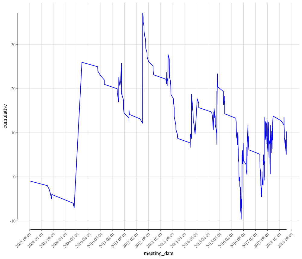
The chart and profit and loss calculations indicate a small profit of 10.31 for a one unit stake across all 377 runners in the dataset. Decent enough, however, we should always ask if this is the full story.
One way of investigating further is to create a scatter plot of the Starting Price for all O’Brien and Moore winners. The ggplot library is again used for this. There are many very powerful features of this charting tool and a wide number of tutorials available online.
# Filter for winners only
obrien_moore_group_races_winners_only <- dplyr::filter(obrien_moore_group_races_only,
                                                       finish_position == 1)

# Scatter plot of winning prices for all O'Brien and Moore winners
ggplot(obrien_moore_group_races_winners_only , aes(x=meeting_date, y=starting_price_decimal)) +
  geom_point(colour="blue") +
  scale_x_date(labels = date_format("%Y-%m-%d"), date_breaks="6 months") +
  theme_tufte(base_family="serif", base_size = 14) +
  theme(axis.text.x = element_text(angle = 45, hjust = 1),
        panel.grid.major.x = element_line(color = "grey80"),
        panel.grid.major.y = element_line(color = "grey80")) +
  geom_smooth(method=loess,
              color="darkred")
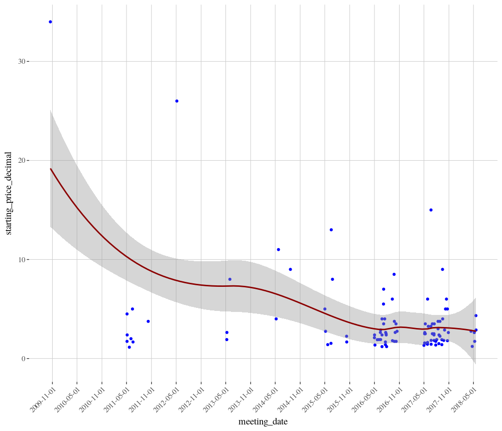
This very interesting chart includes a loess regression line with confidence intervals. The line indicates that the price of O’Brien and Moore winners has been reducing over time, although it also appears that the confidence interval narrows (a good thing!) as the number of rides increases. The slight increase in confidence interval in 2018 is due to the fact the season is not yet half completed and the overall number of runners for this combination is low so far this year.
The chart also clearly shows that the overall Profit and Loss is probably skewed by the big priced winners in 2009 and 2012. If these two rides were removed, the combination would show an overall large loss.
We could also plot every individual runner for this combination, with a separate regression line for both winners and all other runners. In the chart below, winners are the blue points and all other runners are orange.
# Scatter plot of winning prices for all O'Brien and Moore runners
ggplot(obrien_moore_group_races_only , aes(x=meeting_date, y=starting_price_decimal, color=finish_position == 1)) +
  geom_point() +
  scale_x_date(labels = date_format("%Y-%m-%d"),
               date_breaks="12 months") +
  scale_y_continuous(breaks= seq(0,35,by=2)) +
  theme_tufte(base_family="serif",
              base_size = 14) +
  theme(axis.text.x = element_text(angle = 45, hjust = 1),
        panel.grid.major.x = element_line(color = "grey80"),
        panel.grid.major.y = element_line(color = "grey80"),
        legend.position="top") +
  scale_color_manual(values=c("#FF9933","#000CCC")) +
  geom_smooth(method=lm, se=FALSE, fullrange=TRUE)
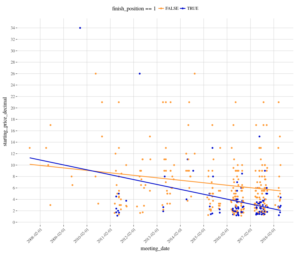
This chart shows that there are tight clusters of winners and runners in 2016 and 2017. We can also see that the starting price of winners has been contracting faster than the overall price of all starters for this combination. As bettors, we should always keep in mind the value proposition of a bet.
Next, we could filter the data and examine just runners from the 2016 season onwards, with a starting price of less than 4.00.
# Filter the data for starters at an SP of less than 4.0 and since 2016 only
obrien_moore_group_races_only_price_filter <- dplyr::filter(obrien_moore_group_races_only,
                                                            starting_price_decimal <= 4.0 &
                                                              meeting_date >= "2016-01-01")

# Calcualte profit and loss
obrien_moore_cumulative <- cumsum(
  ifelse(obrien_moore_group_races_only_price_filter$finish_position == 1, (obrien_moore_group_races_only_price_filter$starting_price_decimal-1),-1)
)

obrien_moore_group_races_only_price_filter$cumulative <- obrien_moore_cumulative

# Plot the results as a line chart
ggplot(data=obrien_moore_group_races_only_price_filter, aes(x=meeting_date, y=cumulative, group=1)) +
  geom_line(colour="blue", lwd=0.7) +
  scale_x_date(labels = date_format("%Y-%m-%d"), date_breaks="6 months") +
  theme_tufte(base_family="serif", base_size = 14) +
  geom_rangeframe() +
  theme(axis.text.x = element_text(angle = 45, hjust = 1),
        panel.grid.major.x = element_line(color = "grey80"),
        panel.grid.major.y = element_line(color = "grey80"))

# Calculate strike rate
winners_only <- nrow(dplyr::filter(obrien_moore_group_races_only_price_filter,
                                    finish_position == 1))

runners <- nrow(obrien_moore_group_races_only_price_filter)

strike_rate <- (winners_only / runners) * 100
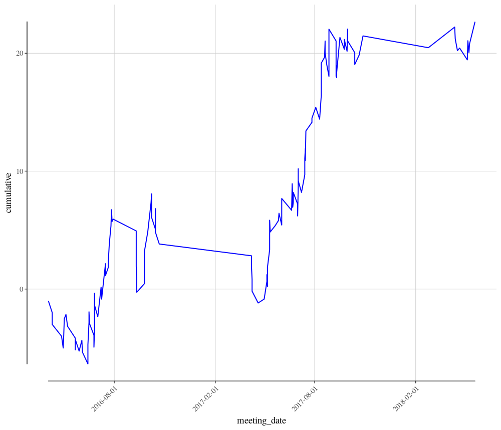
We now have a very healthy 22.67 profit from 133 runners over the last two seasons, with a strike rate of 49.62%. This seems like a quite nice angle into Group races where Aiden O’Brien has a horse ridden by Ryan Moore.
The chart shows that 2016 was a bit slow to begin with, but than picked up nicely from around June onwards. However, 2017 was a very strong year. This year, 2018, seems to be off to a decent start.
There are many other angles which could be investigated. For example, we could filter for:
- Group 1 races only
- Odds on runners only
- Odds between 2.0 and 4.0
- Odds less than 10.0 only
- A distance filter
- A UK vs Ireland scatter chart and filter
There are many, many different ways of investigating further.
Today’s races includes the Irish 2000 Guineas at the Curragh, as well as some other Group races on the same card. Are there any O’Brien and Moore qualifiers?
There are three qualifying horses – US Navy Flag in the Irish 2000 Guineas, Merchant Navy in the Group 2 Greenland Stakes and Hydrangea in the Group 2 Lanwades Stud Stakes, all at prices less than 3/1.
Are all three worth a bet? There’s always something else to consider. Why did Ryan Moore’s number of rides and winners increase markedly from 2016 onwards? In March 2016 Joseph O’Brien announced his retirement from race riding. Ryan Moore most likely then picked up a number of high quality rides which would have otherwise gone to Joseph.
In the 2000 Guineas at Newmarket a few weeks ago, another of Aiden O’Brien’s sons, Donnacha, had a winning ride on Saxon Warrior. This may have only been because Moore was otherwise engaged for Ballydoyle at the Kentucky Derby. What are the current internal dynamics at the stable now? Has Donnacha’s success elevated him in the pecking order?
Donnacha O’Brien rides Gustav Klimt in today’s 2000 Irish Guineas. How important is this race for the stable? Is it an opportunity for Donnacha to ride another Group 1 winner? Of the three qualifying horses today, is it worth considering not betting on US Navy Flag? Racing is never an easy or straightforward game.
Questions and queries about this article should be posted as a comment below or on the Betwise Q&A board.
The full R code used in this article is found below.
# Load the RMySQL library package
library("RMySQL")
library("dplyr")
library("ggplot2")
library("ggthemes")
library("scales")

# Connect to the Smartform database. Substitute the placeholder credentials for your own.
# The IP address can be substituted for a remote location if appropriate.
con <- dbConnect(MySQL(),
                        host='127.0.0.1',
                        user='yourusername',
                        password='yourpassword',
                        dbname='smartform')

sql1 <- paste("SELECT historic_races.course,
              historic_races.meeting_date,
              historic_races.conditions,
              historic_races.group_race,
              historic_races.race_type_id,
              historic_races.race_type,
              historic_runners.name,
              historic_runners.jockey_name,
              historic_runners.trainer_name,
              historic_runners.finish_position,
              historic_runners.starting_price_decimal
              FROM smartform.historic_runners
              JOIN smartform.historic_races USING (race_id)
              WHERE historic_races.meeting_date >= '2006-01-01'", sep="")

smartform_results <- dbGetQuery(con, sql1)

dbDisconnect(con)

# Filter SQL results for flat races only
flat_races_only <- dplyr::filter(smartform_results,
                                 race_type_id == 12 |
                                   race_type_id == 15)
# Filter for Group races only
group_races_only <- dplyr::filter(flat_races_only,
                                  group_race == 1 |
                                    group_race == 2 |
                                    group_race == 3 )

# Filter for Aiden O'Brien runners only
obrien_group_races_only <- dplyr::filter(group_races_only,
                                         grepl("A P O'Brien", trainer_name))

# Remove non-runners
obrien_group_races_only <- dplyr::filter(obrien_group_races_only, !is.na(finish_position))

# Filter for Ryan Moore rides only
obrien_moore_group_races_only <- dplyr::filter(obrien_group_races_only,
                                               grepl("R L Moore", jockey_name))

# Calculate Profit and Loss
obrien_moore_cumulative <- cumsum(
  ifelse(obrien_moore_group_races_only$finish_position == 1, (obrien_moore_group_races_only$starting_price_decimal-1),-1)
)

obrien_moore_group_races_only$cumulative <- obrien_moore_cumulative

# Convert meeting_date columns to Date type
obrien_moore_group_races_only$meeting_date <- as.Date(obrien_moore_group_races_only$meeting_date)

# Plot the results
ggplot(data=obrien_moore_group_races_only, aes(x=meeting_date, y=cumulative, group=1)) +
  geom_line(colour="blue", lwd=0.7) +
  scale_x_date(labels = date_format("%Y-%m-%d"), date_breaks="6 months") +
  theme_tufte(base_family="serif", base_size = 14) +
  geom_rangeframe() +
  theme(axis.text.x = element_text(angle = 45, hjust = 1),
        panel.grid.major.x = element_line(color = "grey80"),
        panel.grid.major.y = element_line(color = "grey80"))

# Filter for winners only
obrien_moore_group_races_winners_only <- dplyr::filter(obrien_moore_group_races_only,
                                                       finish_position == 1)

# Scatter plot of winning prices for all O'Brien and Moore winners
ggplot(obrien_moore_group_races_winners_only , aes(x=meeting_date, y=starting_price_decimal)) +
  geom_point(colour="blue") +
  scale_x_date(labels = date_format("%Y-%m-%d"), date_breaks="6 months") +
  theme_tufte(base_family="serif", base_size = 14) +
  theme(axis.text.x = element_text(angle = 45, hjust = 1),
        panel.grid.major.x = element_line(color = "grey80"),
        panel.grid.major.y = element_line(color = "grey80")) +
  geom_smooth(method=loess,
              color="darkred")

# Scatter plot of winning prices for all O'Brien and Moore runners
ggplot(obrien_moore_group_races_only , aes(x=meeting_date, y=starting_price_decimal, color=finish_position == 1)) +
  geom_point() +
  scale_x_date(labels = date_format("%Y-%m-%d"),
               date_breaks="12 months") +
  scale_y_continuous(breaks= seq(0,35,by=2)) +
  theme_tufte(base_family="serif",
              base_size = 14) +
  theme(axis.text.x = element_text(angle = 45, hjust = 1),
        panel.grid.major.x = element_line(color = "grey80"),
        panel.grid.major.y = element_line(color = "grey80"),
        legend.position="top") +
  scale_color_manual(values=c("#FF9933","#000CCC")) +
  geom_smooth(method=lm, se=FALSE, fullrange=TRUE)

# Filter the data for starters at an SP of less than 4.0 and since 2016 only
obrien_moore_group_races_only_price_filter <- dplyr::filter(obrien_moore_group_races_only,
                                                            starting_price_decimal <= 4.0 &
                                                              meeting_date >= "2016-01-01")

# Calcualte profit and loss
obrien_moore_cumulative <- cumsum(
  ifelse(obrien_moore_group_races_only_price_filter$finish_position == 1, (obrien_moore_group_races_only_price_filter$starting_price_decimal-1),-1)
)

obrien_moore_group_races_only_price_filter$cumulative <- obrien_moore_cumulative

# Plot the results as a line chart
ggplot(data=obrien_moore_group_races_only_price_filter, aes(x=meeting_date, y=cumulative, group=1)) +
  geom_line(colour="blue", lwd=0.7) +
  scale_x_date(labels = date_format("%Y-%m-%d"), date_breaks="6 months") +
  theme_tufte(base_family="serif", base_size = 14) +
  geom_rangeframe() +
  theme(axis.text.x = element_text(angle = 45, hjust = 1),
        panel.grid.major.x = element_line(color = "grey80"),
        panel.grid.major.y = element_line(color = "grey80"))

# Calculate strike rate
winners_only <- nrow(dplyr::filter(obrien_moore_group_races_only_price_filter,
                                    finish_position == 1))

runners <- nrow(obrien_moore_group_races_only_price_filter)

strike_rate <- (winners_only / runners) * 100